Reviewing one year of blogging

Writing blog posts has been one of the most rewarding experiences for me over the last year. Some posts turned out quite long, others I could keep more concise. Irrespective of length, however, I have managed to publish one post every month, and you can infer the occassional frenzy that ensued from the distribution of the dates the posts appeared on — nine of them saw the light within the last three days of a month.

Some births were easier than others, yet every post evokes distinct memories: of perusing history books in the library and the Saturday sun; of writing down Gaussian integrals in overcrowded trains; of solving differential equations while singing; of hunting down typos before hurrying to parties. So to end this very productive year of blogging, below I provide a teaser of each previous post, summarizing one or two key takeaways. Let’s go!

An introduction to Causal inference

Causal inference goes beyond prediction by modeling the outcome of interventions and formalizing counterfactual reasoning. It dethrones randomized control trials as the only tool to license causal statements, describing the conditions under which this feat is possible even in observational data.

One key takeaway is to think about causal inference in a hierarchy. Association is at the most basic level, merely allowing us to say that two variables are somehow related. Moving upwards, the do-operator allows us to model interventions, answering questions such as “what would happen if we force every patient to take the drug”? Directed Acyclic Graphs (DAGs), as visualized in the figure below, allow us to visualize associations and causal relations.

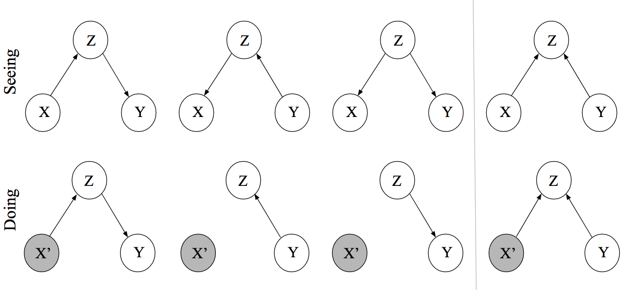
On the third and final level we find counterfactual statements. These follow from so-called Structural Causal Models — the building block of this approach to causal inference. Counterfactuals allow us to answer questions such as “would the patient have recovered had she been given the drug, even though she has not received the drug and did not recover”? Needless to say, this requires strong assumptions; yet if we want to endow machines with human-level reasoning or formalize concepts such as fairness, we need to make such strong assumptions.

One key practical take a way from this blog post is the definition of confounding: an effect is confounded if $p(Y \mid X) \neq p(Y \mid do(X = x))$. This means that blindly entering all variables into a regression to “control” for them is misguided; instead, one should carefuly think about the underlying causal relations between variables so as to not induce spurious associations. You can read the full blog post here.

A brief primer on Variational Inference

Bayesian inference using Markov chain Monte Carlo can be notoriously slow. The key idea behind variational inference is to recast Bayesian inference as an optimization problem. In particular, we try to find a distribution $q^\star(\mathbf{z})$ that best approximates the posterior distribution $p(\mathbf{z} \mid \mathbf{x})$ in terms of the Kullback-Leibler divergence:

\[q^\star(\mathbf{z}) = \underbrace{\text{argmin}}_{q(\mathbf{z}) \in \mathrm{Q}} \text{ KL}\left(q(\mathbf{z}) \, \lvert\lvert \, p(\mathbf{z} \mid \mathbf{x}) \right) \enspace .\]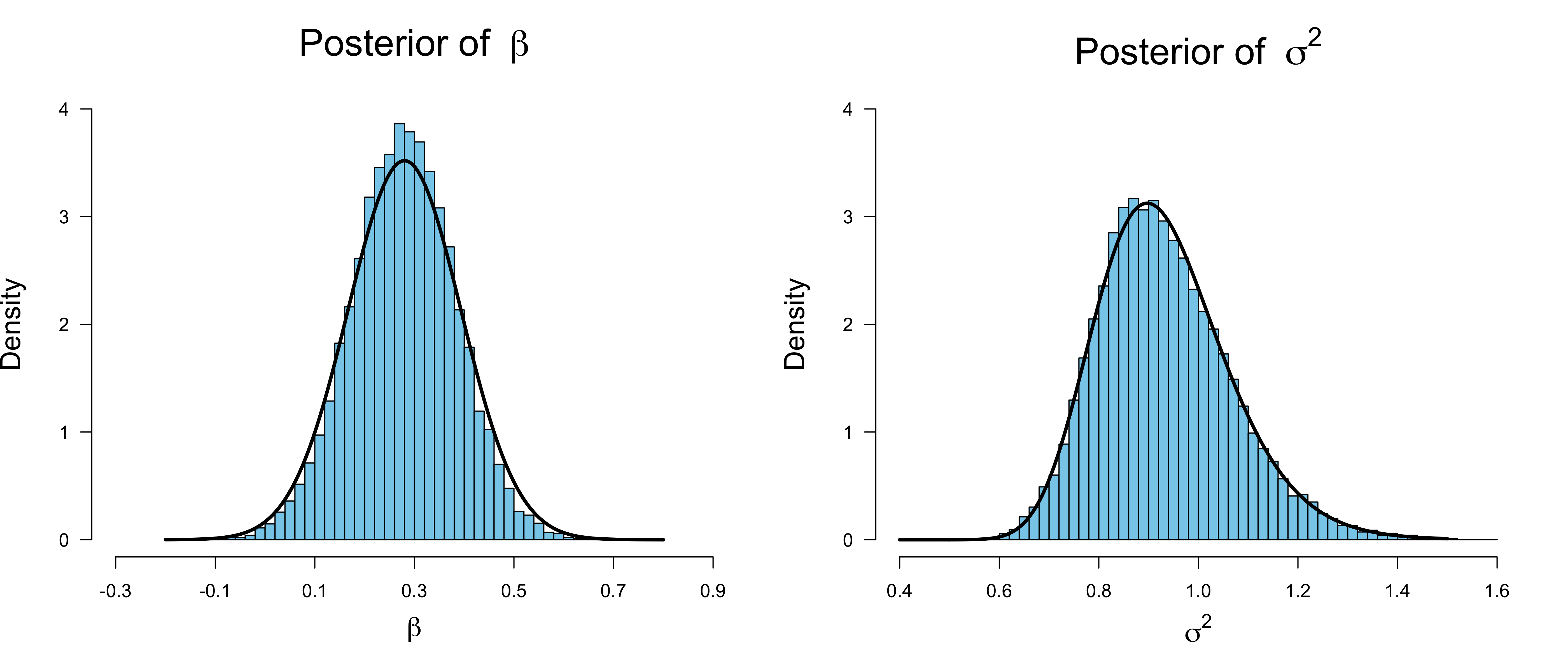

In this blog post, I explain how a particular form of variational inference — coordinate ascent mean-field variational inference — leads to fast computations. Specifically, I walk you through deriving the variational inference scheme for a simple linear regression example. One key takeaway from this post is that Bayesians can use optimization to speed up computation. However, variational inference requires problem-specific, often tedious calculations. Black-box variational inference schemes can alleviate this issue, but Stan’s implementation — automatic differentiation variational inference — seems to work poorly, as detailed in the post (see also Ben Goodrich’s comment). You can read the full blog post here.

Harry Potter and the Power of Bayesian Constrained Inference

Are you a Gryffindor, Slytherin, Hufflepuff, or Ravenclaw? In this blog post, I explain a prior predictive perspective on model selection by having Harry, Ron, and Hermione — three subjective Bayesians — engage in a small prediction contest. There are two key takeaways. First, the prior does not completely constrain a model’s prediction, as these are being made by combining the prior with the likelihood. For example, even though Ron has a point prior on $\theta = 0.50$ in the figure below, his prediction is not that $y = 5$ always; instead, he predicts a distribution that is centered around $y = 5$. Similarly, while Hermione believes that $\theta > 0.50$, she puts probability mass on values $y < 5$.

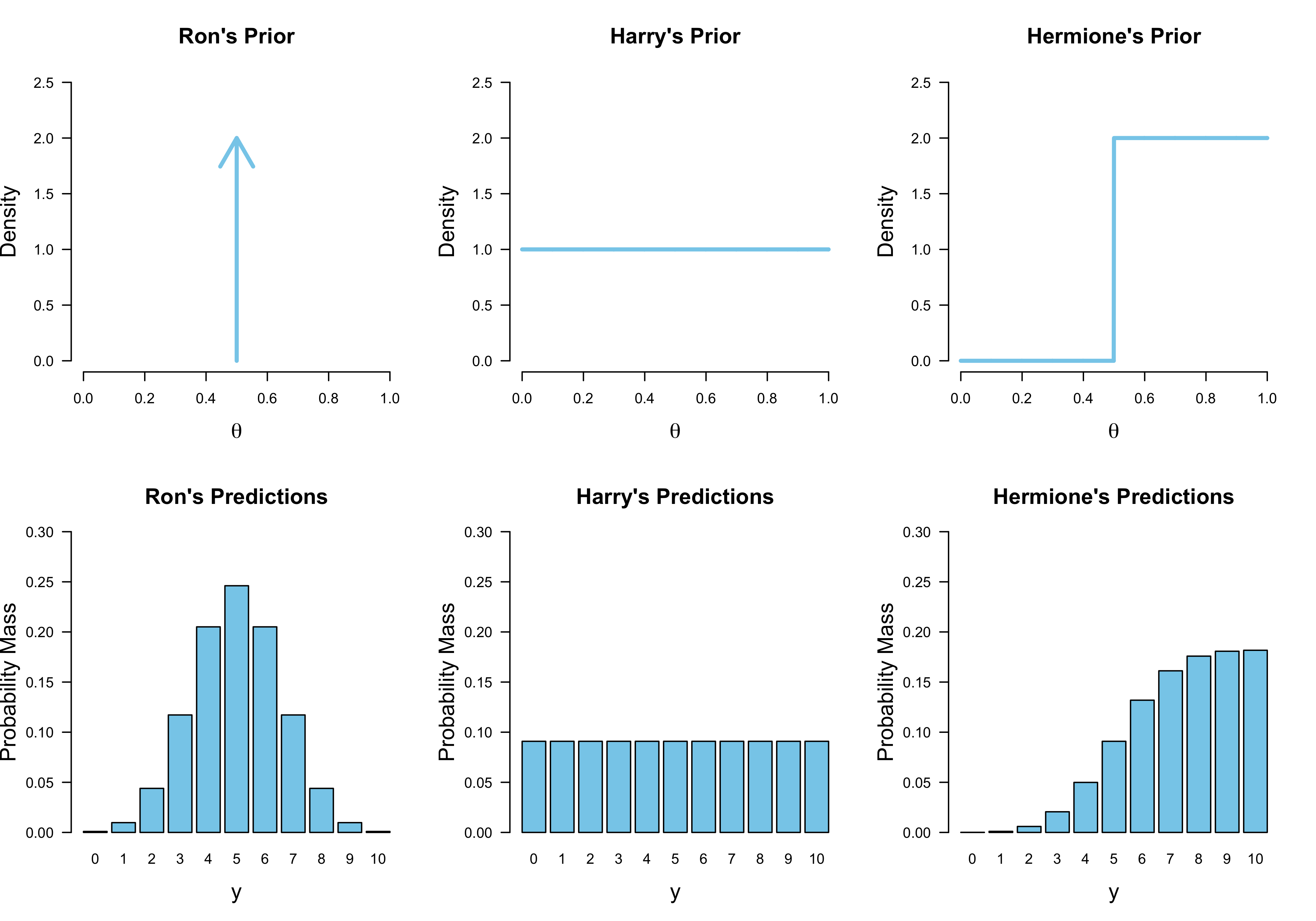
The second takeaway is computational. In particular, one can compute the Bayes factor of the unconstrained model ($\mathcal{M}_1$) — in which the parameter $\theta$ is free to vary — against a constrained model ($\mathcal{M}_r$) — in which $\theta$ is order-constrained (e.g., $\theta > 0.50$) — as:

\[\text{BF}_{r1} = \frac{p(\theta \in [0.50, 1] \mid y, \mathcal{M}_1)}{p(\theta \in [0.50, 1] \mid \mathcal{M}_1)} \enspace .\]

In words, this Bayes factor is given by the ratio of the posterior probability of $\theta$ being in line with the restriction compared to the prior probability of $\theta$ being in line with the restriction. You can read the full blog post here.

Love affairs and linear differential equations

When you can fall for chains of silver, you can fall for chains of gold
You can fall for pretty strangers and the promises they hold
You promised me everything, you promised me thick and thin, yeah
Now you just say "Oh, Romeo, yeah, you know I used to have a scene with him"

Differential equations are the sine qua non of modeling how systems change. This blog post provides an introduction to linear differential equations, which admit closed-form solutions, and analyzes the stability of fixed points.

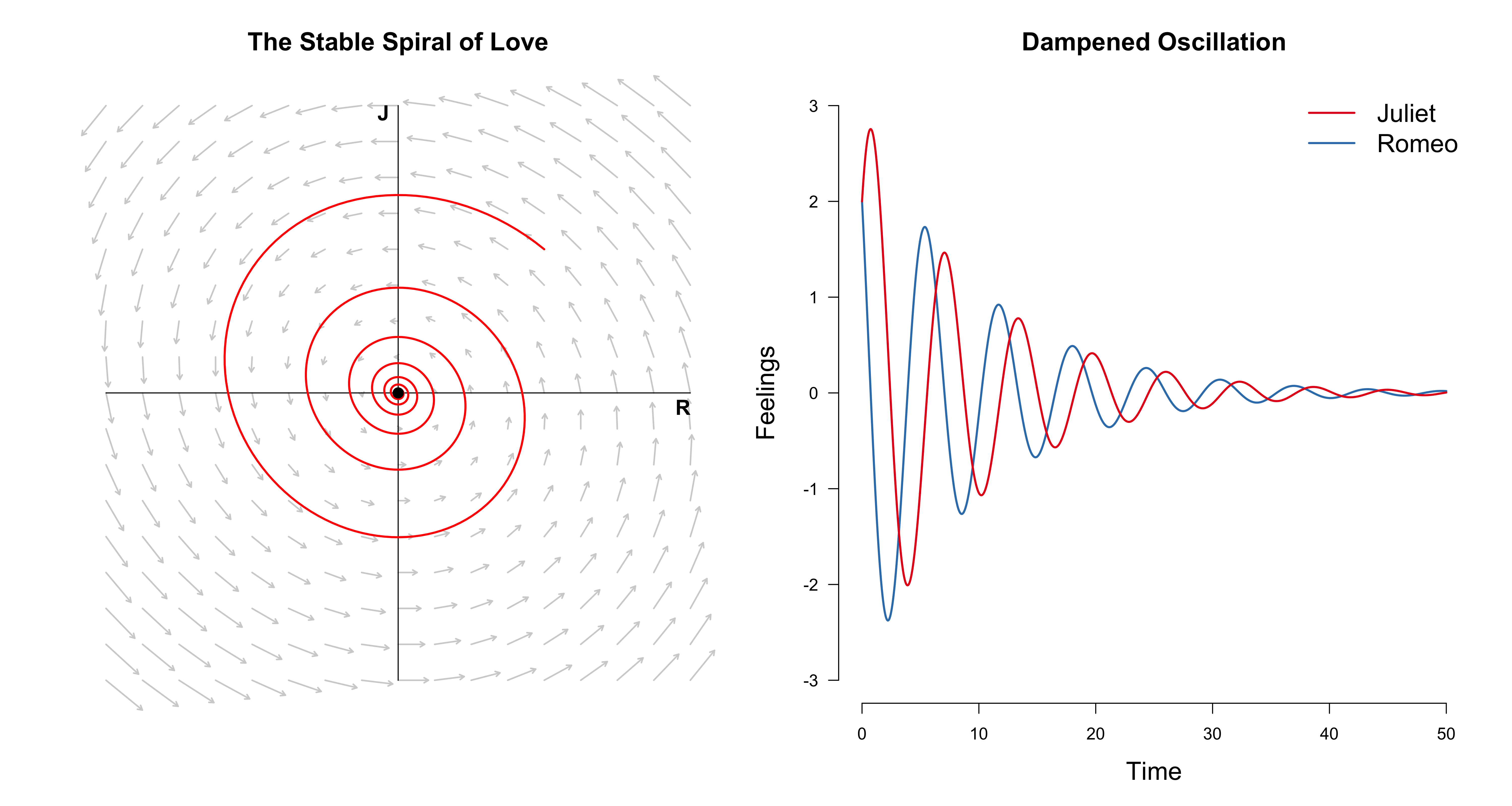
The key takeaways are that the natural basis of analysis is the basis spanned by the eigenvectors, and that the stability of fixed points depends directly on the eigenvalues. A system with imaginary eigenvalues can exhibit oscillating behaviour, as shown in the figure above.

I think I rarely had more fun writing than when writing this blog post. Inspired by Strogatz (1988), it playfully introduces linear differential equations by classifying the types of relationships Romeo and Juliet might find themselves in. While writing it, I also listened to a lot of Dire Straits, Bob Dylan, Daft Punk, and others, whose lyrics decorate the post’s section. You can read the full blog post here.

The Fibonacci sequence and linear algebra

1, 1, 2, 3, 5, 8, 13, 21, … The Fibonacci sequence might well be the most widely known mathematical sequence. In this blog post, I discuss how Leonardo Bonacci derived it as a solution to a puzzle about procreating rabbits, and how linear algebra can help us find a closed-form expression of the $n^{\text{th}}$ Fibonacci number.

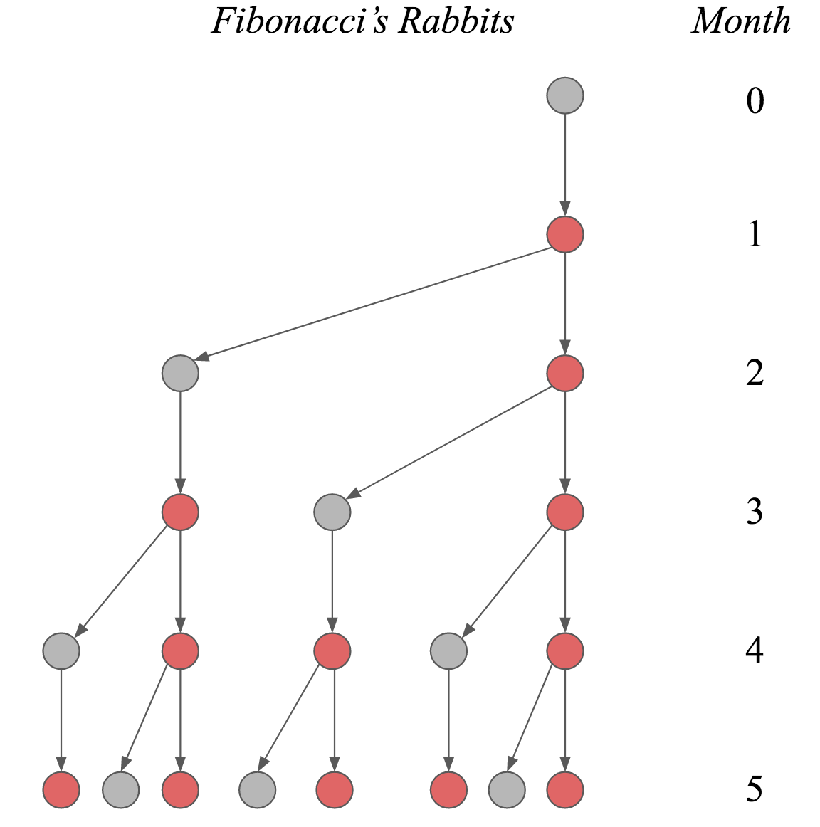
The key insight is to realize that the $n^{\text{th}}$ Fibonacci number can be computed by repeatedly performing matrix multiplications. If one diagonalizes this matrix, changing basis to — again! — the eigenbasis, then the repeated application of this matrix can be expressed as a scalar power, yielding a closed-form expression of the $n^{\text{th}}$ Fibonacci number. That’s a mouthful; you can read the blog post which explains things much better here.

Spurious correlations and random walks

I was at the Santa Fe Complex Systems Summer School — the experience of a lifetime — when Anton Pichler and Andrea Bacilieri, two economists, told me that two independent random walks can be correlated substantially. I was quite shocked, to be honest. This blog post investigates this issue, concluding that regressing one random walk onto another is nonsensical, that is, leads to an inconsistent parameter estimate.

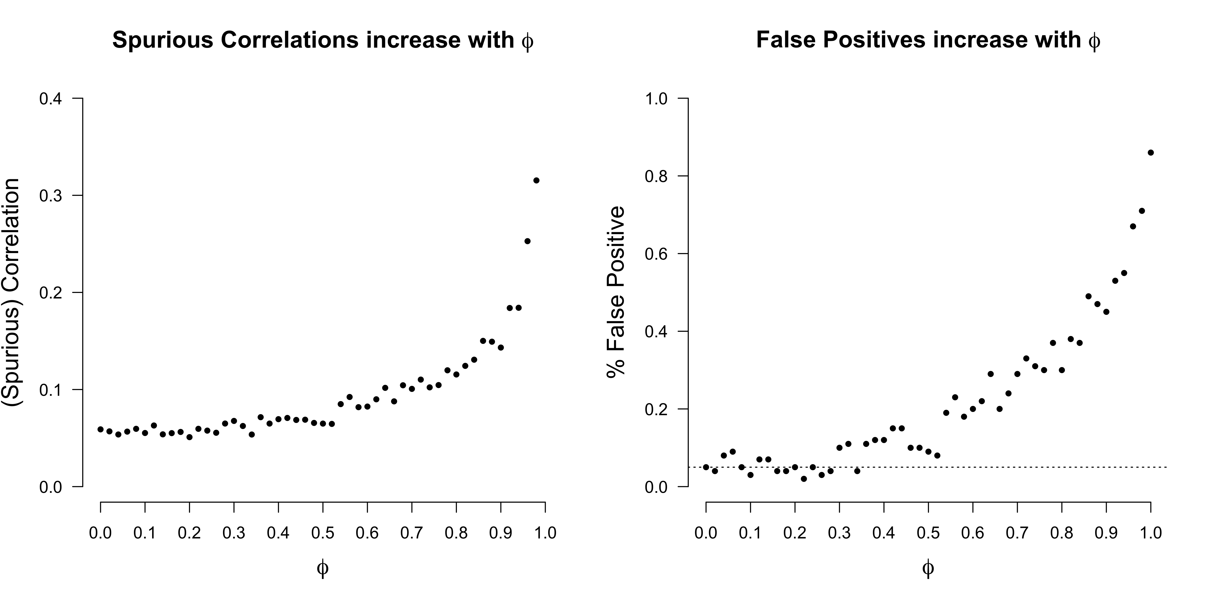
As the figure above shows, such spurious correlation also occurs for independent AR(1) processes with increasing autocorrelation $\phi$, even though the resulting estimate is consistent. The key takeaway is therefore to be careful when correlating time-series. You can read the full blog post here.

Bayesian modeling using Stan: A case study

Model selection is a difficult problem. In Bayesian inference, we may distinguish between two approaches to model selection: a (prior) predictive perspective based on marginal likelihoods, and a (posterior) predictive perspective based on leave-one-out cross-validation.

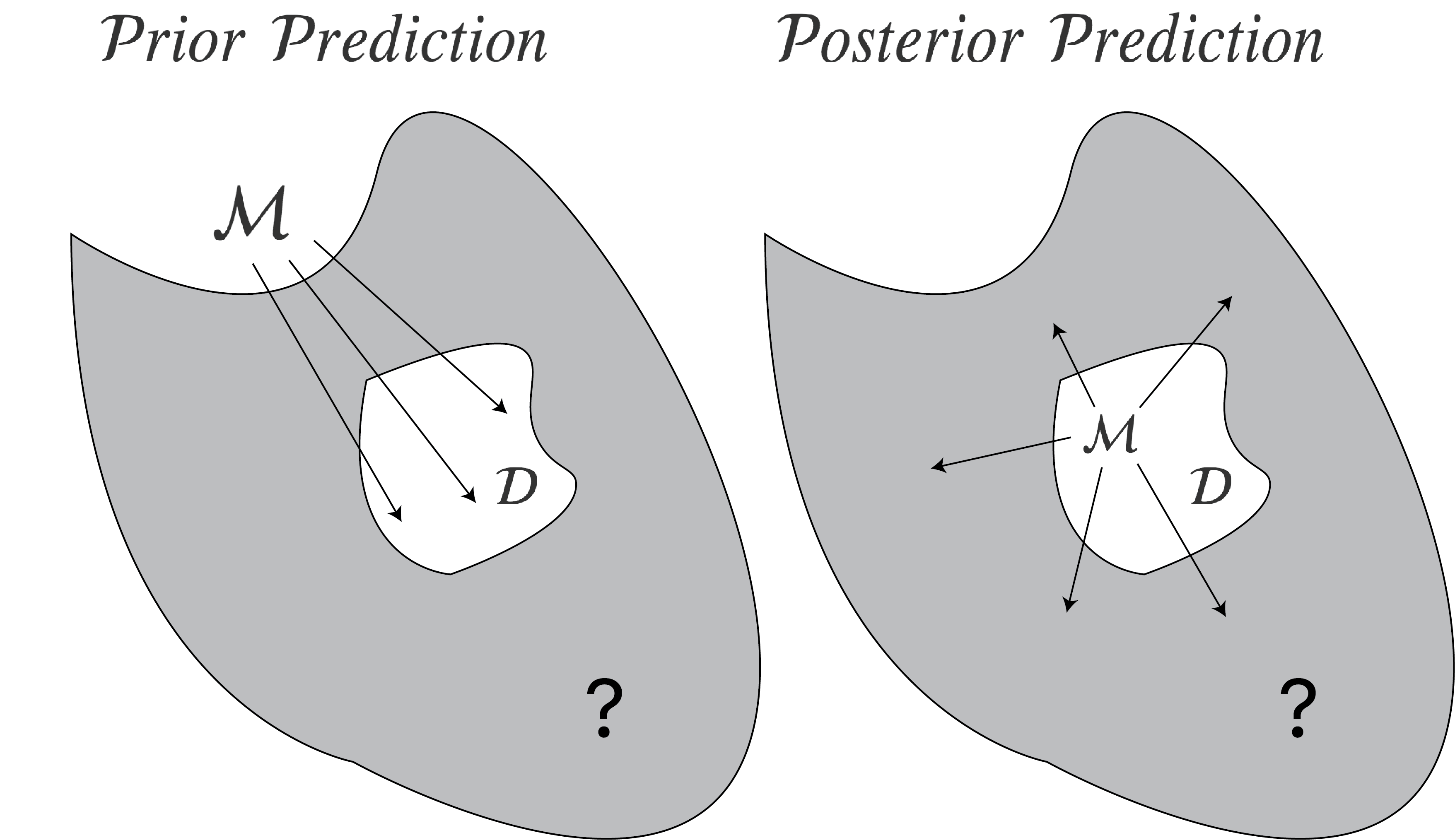
A prior predictive perspective — illustrated in the left part of the figure above — evaluates models based on their predictions about the data actually observed. These predictions are made by combining likelihood and prior. In contrast, a posterior predictive perspective — illustrated in the right panel of the figure above — evaluates models based on their predictions about data that we have not observed. These predictions cannot be directly computed, but can be approximated by combining likelihood and posterior in a leave-one-out cross-validation scheme. They key takeaway of this blog post is to appreciate this distinction, noting that not all Bayesians agree on how to select among models.

The post illustrates these two perspectives with a case study: does the relation between practice and reaction time follow a power law or an exponential function? You can read the full blog post here.

Two perspectives on regularization

Regularization is the process of adding information to an estimation problem so as to avoid extreme estimates. This blog post explores regularization both from a Bayesian and from a classical perspective, using the simplest example possible: estimating the bias of a coin.

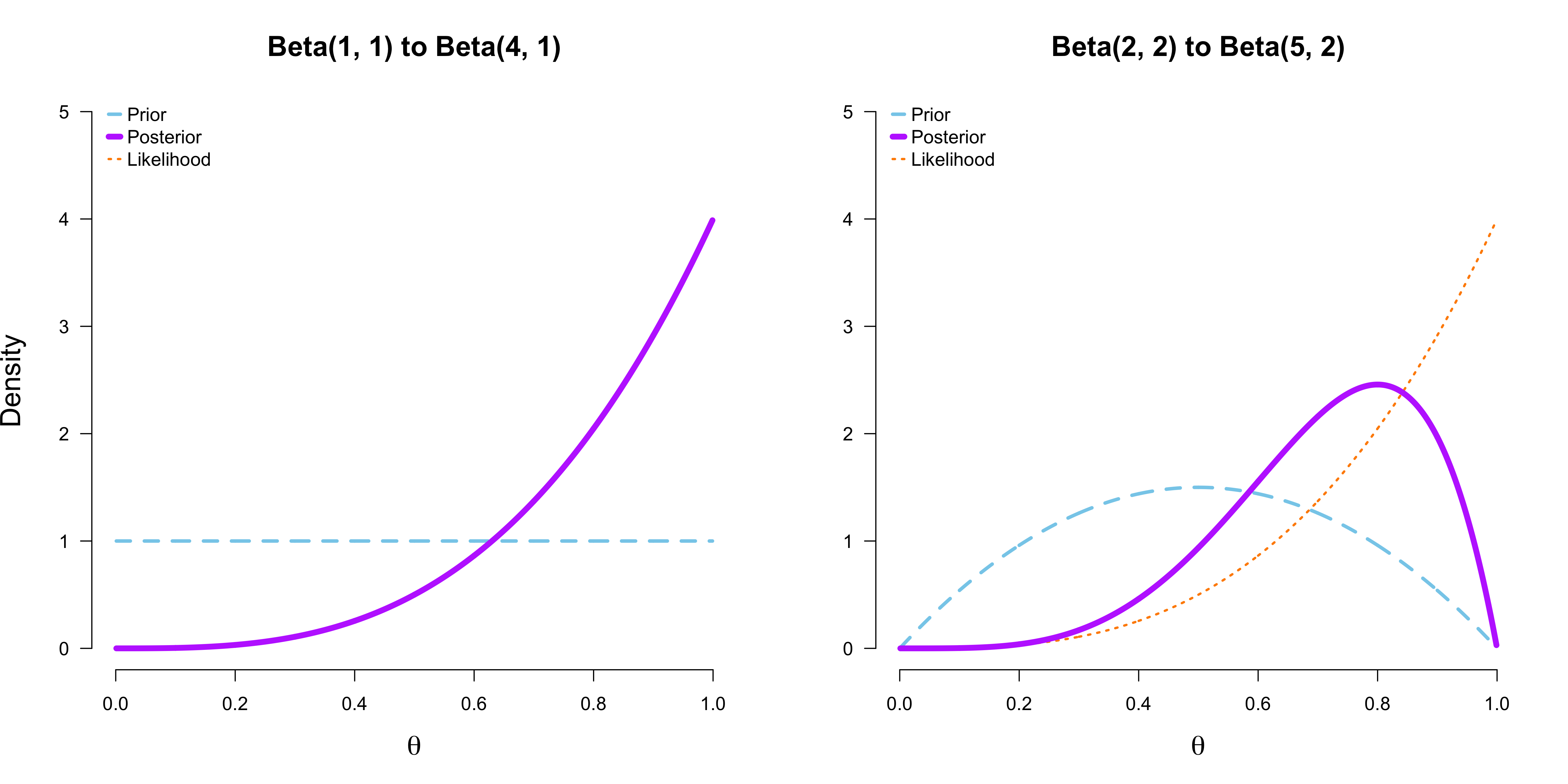
The key takeaway is the observation that Bayesians have a natural tool for regularization at their disposal: the prior. In contrast to the left panel in the figure above, which shows a flat prior, the right panel illustrates that using a weakly informative prior that peaks at $\theta = 0.50$ shifts the resulting posterior distribution towards that value. In classical statistics, one usually uses penalized maximum likelihood approaches — think lasso and ridge regression — to achieve regularization. You can read the full blog post here.

Variable selection using Gibbs sampling

“Which variables are important?” is a key question in science and statistics. In this blog post, I focus on linear models and discuss a Bayesian solution to this problem using spike-and-slab priors and the Gibbs sampler, a computational method to sample from a joint distribution using only conditional distributions.

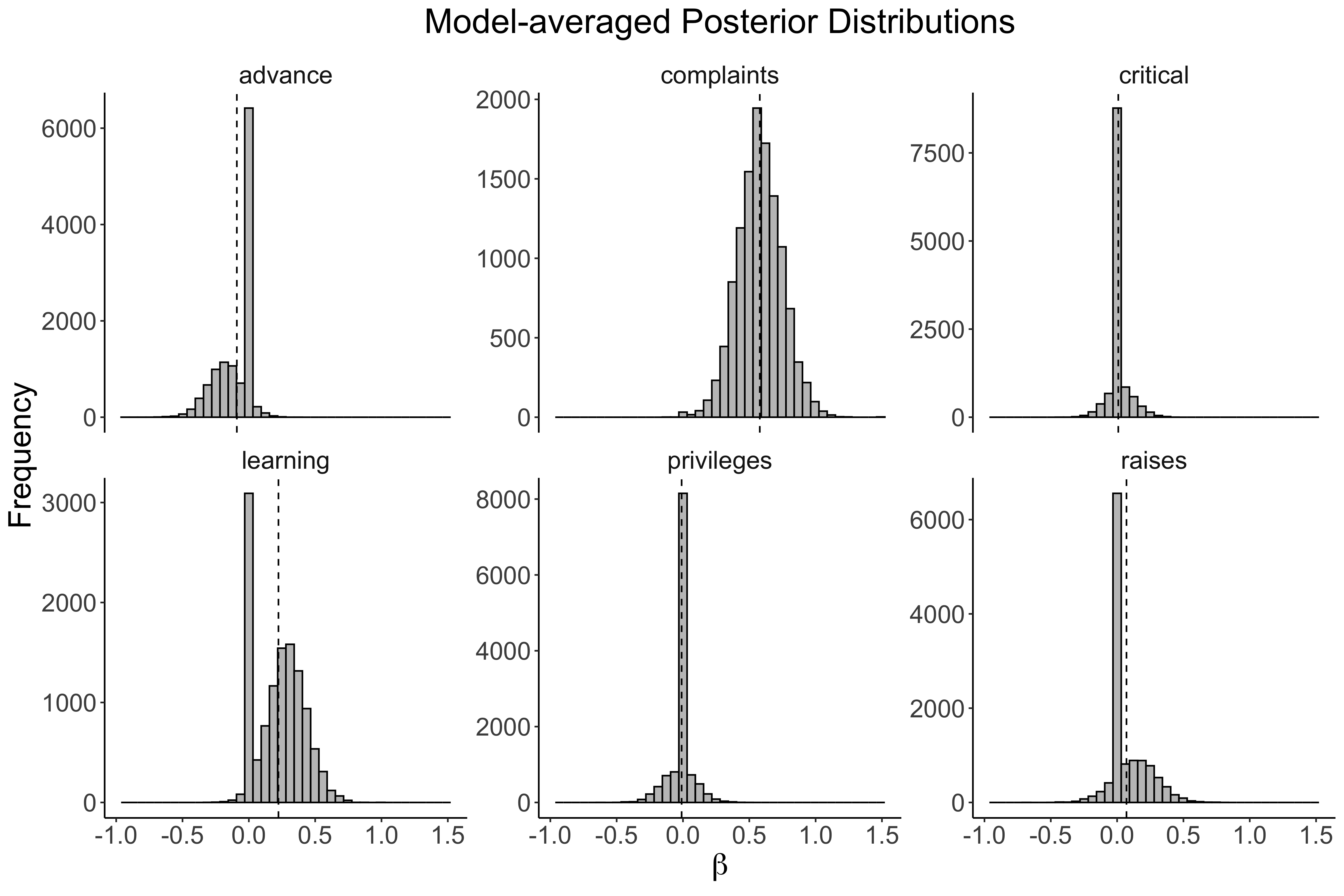
Parameter estimation is almost always conditional on a specific model. One key takeaway from this blog post is that there is uncertainty associated with the model itself. The approach outlined in the post accounts for this uncertainty by using spike-and-slab priors, yielding posterior distributions not only for parameters but also for models. To incorporate this model uncertainty into parameter estimation, one can average across models; the figure above shows the model-averaged posterior distribution for six variables discussed in the post. You can read the full blog post here.

Two properties of the Gaussian distribution

The Gaussian distribution is special for a number of reasons. In this blog post, I focus on two such reasons, namely the fact that it is closed under marginalization and conditioning. This means that if you start out with a p-dimensional Gaussian distribution, and you either marginalize over or condition on one of its components, the resulting distribution will again be Gaussian.

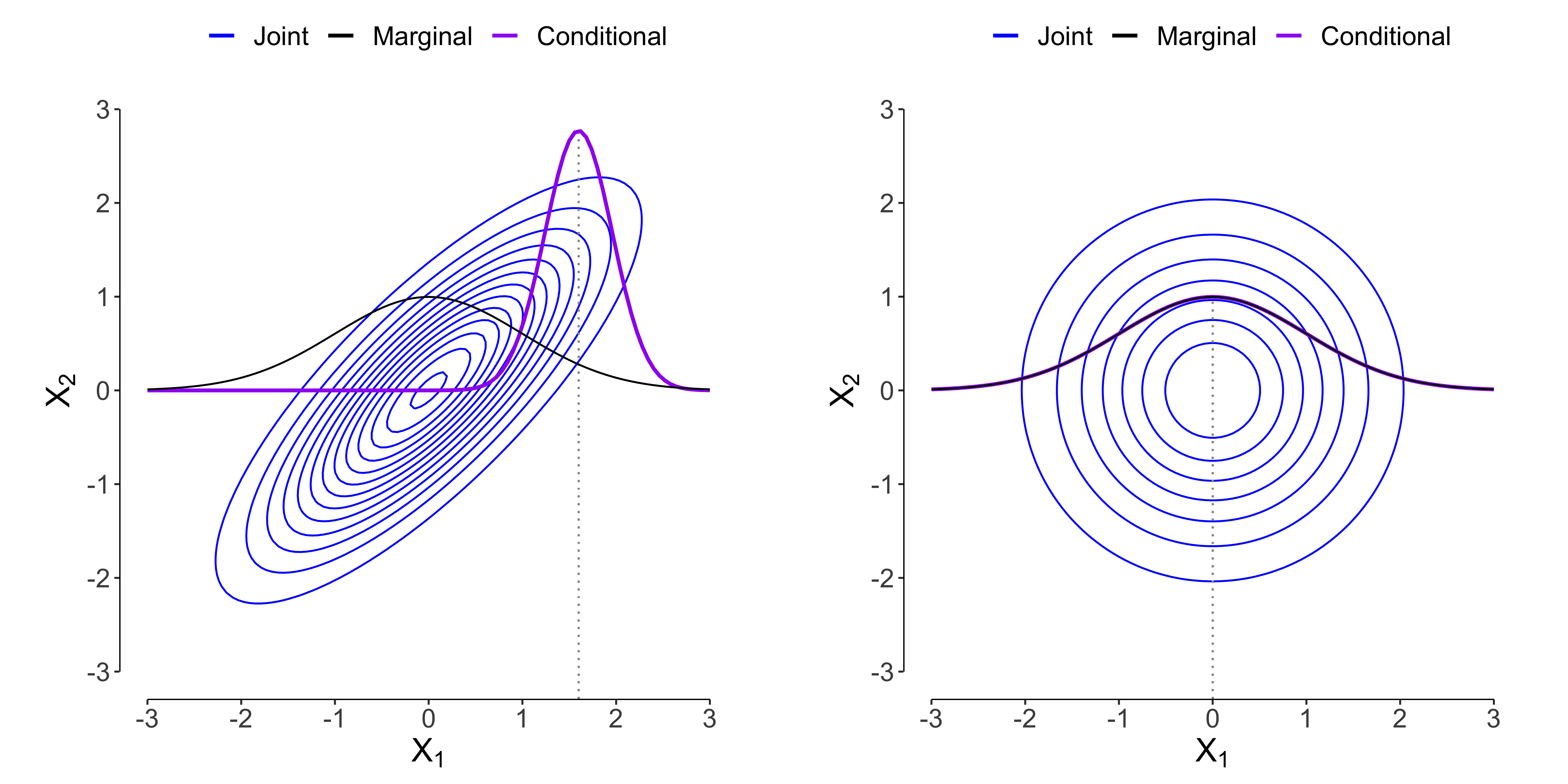
The figure above illustrates the difference between marginalization and conditioning in the two-dimensional case. The left panel shows a bivariate Gaussian distribution with a high correlation $\rho = 0.80$ (blue contour lines). Conditioning means incorporating information, and observing that $X_2 = 2$ shifts the distribution of $X_1$ towards this value (purple line). If we do not observe $X_2$, we can incorporate our uncertainty about its likely values by marginalizing it out. This results in a Gaussian distribution that is centered on zero (black line). The right panel shows that conditioning on $X_2 = 2$ does not change the distribution of $X_1$ in the case of no correlation $\rho = 0$. You can read the full blog post here.

Curve fitting and the Gaussian distribution

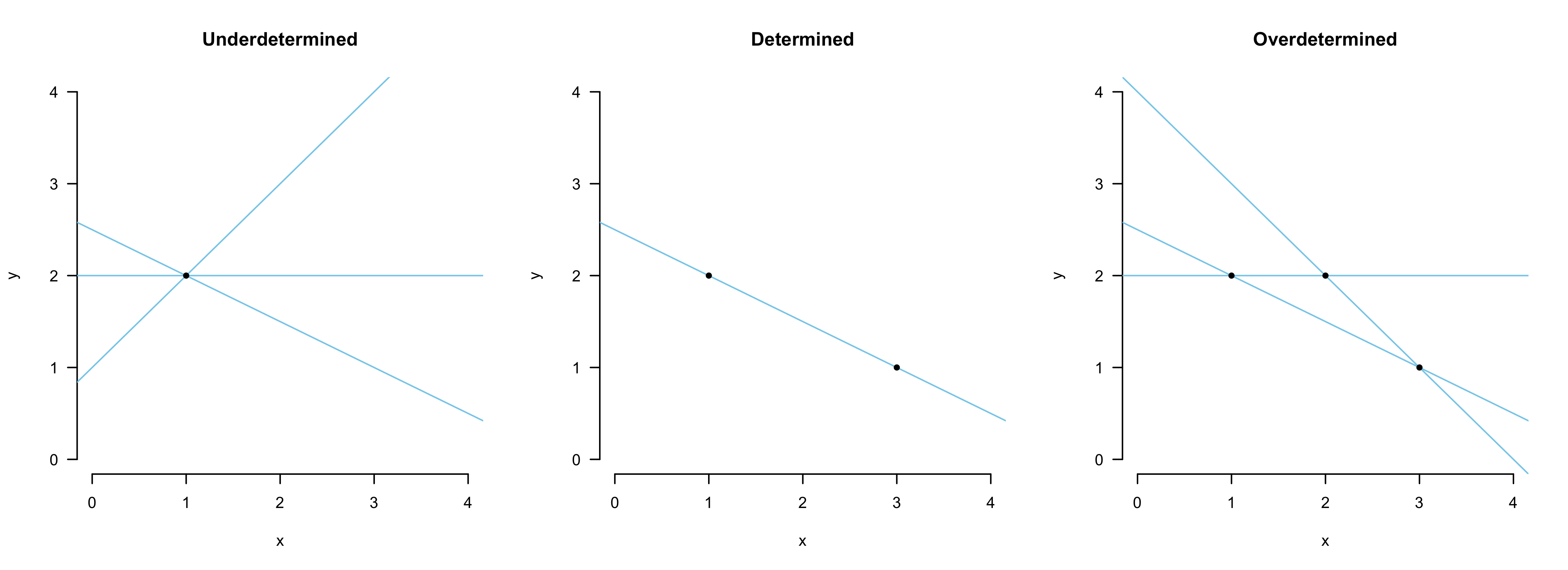
In this blog post, we take a look at the mother of all curve fitting problems — fitting a straight line to a number of points. The figure below shows that one point in the Euclidean plane is insufficient to define a line (left), two points constrain it perfectly (middle), and three is too much (right). In science we usually deal with more than two data points which are corrupted by noise. How do we fit a line to such noisy observations?

The methods of least squares provides an answer. In addition to an explanation of least squares, a key takeaway of this post is an understanding for the historical context in which least squares arose. Statistics is fascinating in part because of its rich history. On our journey through time we meet Legendre, Gauss, Laplace, and Galton. The latter describes the central limit theorem — one of the most stunning theorems in statistics — in beautifully poetic words:

“I know of scarcely anything so apt to impress the imagination as the wonderful form of cosmic order expressed by the “Law of Frequency of Error”. The law would have been personified by the Greeks and deified, if they had known of it. It reigns with serenity and in complete self-effacement, amidst the wildest confusion. The huger the mob, and the greater the apparent anarchy, the more perfect is its sway. It is the supreme law of Unreason. Whenever a large sample of chaotic elements are taken in hand and marshalled in the order of their magnitude, an unsuspected and most beautiful form of regularity proves to have been latent all along.” (Galton, 1889, p. 66)

You can read the full blog post here.

I hope that you enjoyed reading some of these posts at least a quarter as much as I enjoyed writing them. I am committed to making 2020 a successful year of blogging, too. However, I will most likely decrease the output frequency by half, aiming to publish one post every two months. It is a truth universally acknowledged that a person in want of a PhD must be in possession of publications, and so I will have to shift my focus accordingly (at least a little bit). At the same time, I also want to further increase my involvement in the “data for the social good” scene. Life certainly is one complicated optimization problem. I wish you all the best for the new year!

---

I would like to thank Don van den Bergh, Sophia Crüwell, Jonas Haslbeck, Oisín Ryan, Lea Jakob, Quentin Gronau, Nathan Evans, Andrea Bacilieri, and Anton Pichler for helpful comments on (some of) these blog posts.

Written on December 27th, 2019 by Fabian Dablander