Spurious correlations and random walks

The number of storks and the number of human babies delivered are positively correlated (Matthews, 2000). This is a classic example of a spurious correlation which has a causal explanation: a third variable, say economic development, is likely to cause both an increase in storks and an increase in the number of human babies, hence the correlation.¹ In this blog post, I discuss a more subtle case of spurious correlation, one that is not of causal but of statistical nature: completely independent processes can be correlated substantially.

AR(1) processes and random walks

Moods, stockmarkets, the weather: everything changes, everything is in flux. The simplest model to describe change is an auto-regressive (AR) process of order one. Let $Y_t$ be a random variable where $t = [1, \ldots T]$ indexes discrete time. We write an AR(1) process as:

where $\phi$ gives the correlation with the previous observation, and where $\epsilon_t \sim \mathcal{N}(0, \sigma^2)$. For $\phi = 1$ the process is called a random walk. We can simulate from these using the following code:

simulate_ar <- function(n, phi, sigma = .1) {
  y <- rep(0, n)
  
  for (t in seq(2, n)) {
    y[t] <- phi*y[t-1] + rnorm(1, 0, sigma)
  }
  
  y
}

The following R code simulates data from three independent random walks and an AR(1) process with $\phi = 0.5$; the Figure below visualizes them.

n <- 100
set.seed(1)
 
rw1 <- simulate_ar(n, phi = 1)
rw2 <- simulate_ar(n, phi = 1)
rw3 <- simulate_ar(n, phi = 1)
ar <- simulate_ar(n, phi = 0.5)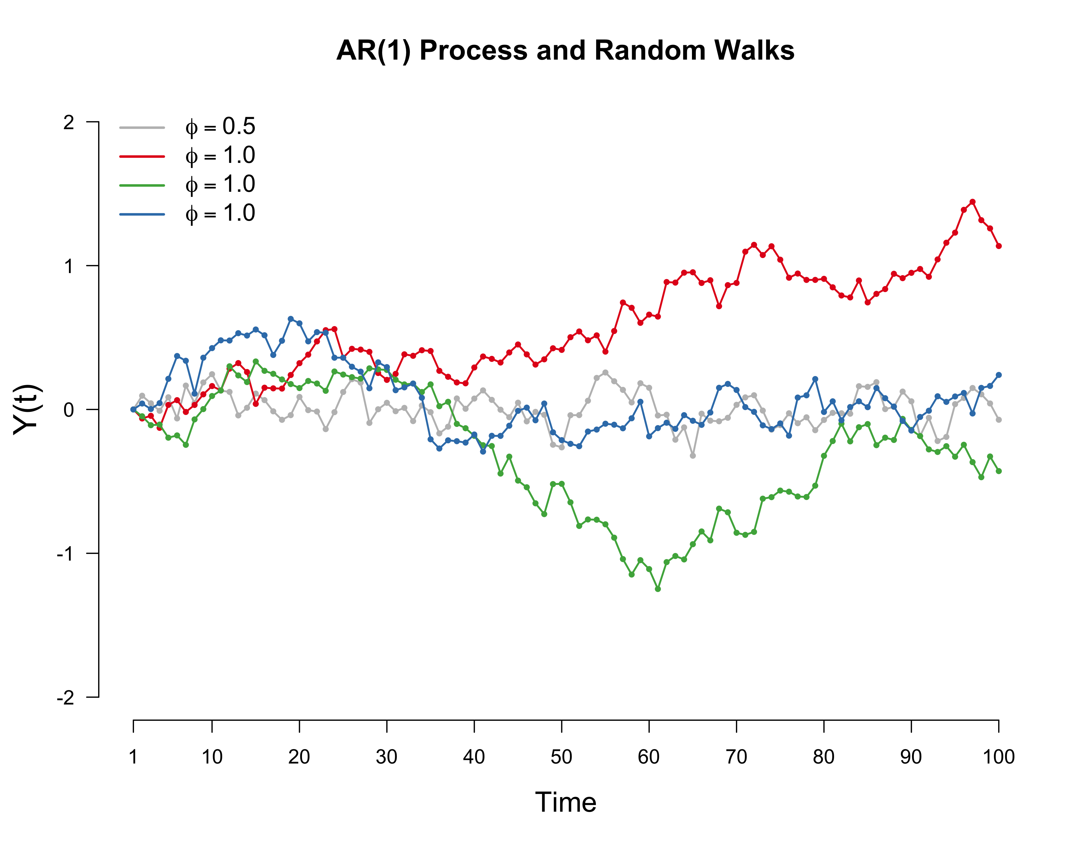

As we can see from the plot, the AR(1) process seems pretty well-behaved. This is in contrast to the three random walks: all of them have an initial upwards trend, after which the red line keeps on growing, while the blue line makes a downward jump. In contrast to AR(1) processes, random walks are not stationary since their variance is not constant across time. For some very good lecture notes on time-series analysis, see here.

Spurious correlations of random walks

If we look at the correlations of these three random walks across time points, we find that they are substantial:

round(cor(cbind(red = rw1, green = rw2, blue = rw3)), 2)

##         red green  blue
## red    1.00 -0.49 -0.29
## green -0.49  1.00  0.59
## blue  -0.29  0.59  1.00

I hope that this is at least a little bit of a shock. Upon reflection, however, it is clear that we are blundering: computing the correlation across time ignores the dependency between data points that is so typical of time-series data. To get more data about what is going on, we conduct a small simulation study.

In particular, we want to get an intuition of how this spurious correlation behaves with increasing sample sizes. We therefore simulate two independent random walks for sample sizes $n \in [50, 100, 200, 500, 1000, 2000]$ and compute their Pearson correlation, the test-statistic, and whether $p < \alpha$, where we set $\alpha$ to some an arbitrary value, say $\alpha = 0.05$. We repeated this 100 times and report the average of these quantities.

library('dplyr')
set.seed(1)
 
times <- 100
ns <- c(50, 100, 200, 500, 1000, 2000)
 
comb <- expand.grid(times = seq(times), n = ns)
ncomb <- nrow(comb)
 
res <- matrix(NA, nrow = ncomb, ncol = 5)
colnames(res) <- c('ix', 'n', 'cor', 'tstat', 'pval')
 
for (i in seq(ncomb)) {
  n <- comb[i, 2]
  ix <- comb[i, 1]
  test <- cor.test(simulate_ar(n, phi = 1), simulate_ar(n, phi = 1))
  res[i, ] <- c(ix, n, test$estimate, test$statistic, test$p.value)
}
 
tab <- data.frame(res) %>% 
  group_by(n) %>% 
  summarize(
    avg_abs_corr = mean(abs(cor)),
    avg_abs_tstat = mean(abs(tstat)),
    percent_sig = mean(pval < .05)
  ) %>% data.frame
 
round(tab, 2)

##      n avg_abs_corr avg_abs_tstat percent_sig
## 1   50         0.41          3.57        0.71
## 2  100         0.46          6.58        0.85
## 3  200         0.45          8.88        0.85
## 4  500         0.37         10.63        0.86
## 5 1000         0.41         17.05        0.88
## 6 2000         0.39         23.39        0.97

We observe that the average absolute correlation is very similar across $n$, but the test statistic grows with increased $n$, which naturally results in many more false rejections of the null hypothesis of no correlation between the two random walks.

To my knowledge, Granger and Newbold (1974) were the first to point out this puzzling fact.² They regress one random walk onto the other instead of computing the Pearson correlation. (Note that the test statistic is the same). In a regression setting, we write:

where we assume that $\epsilon_i \sim \mathcal{N}(0, \sigma^2)$ (see also a previous blog post). This is evidently violated when performing linear regression on two random walks, as demonstrated by the residual plot below.

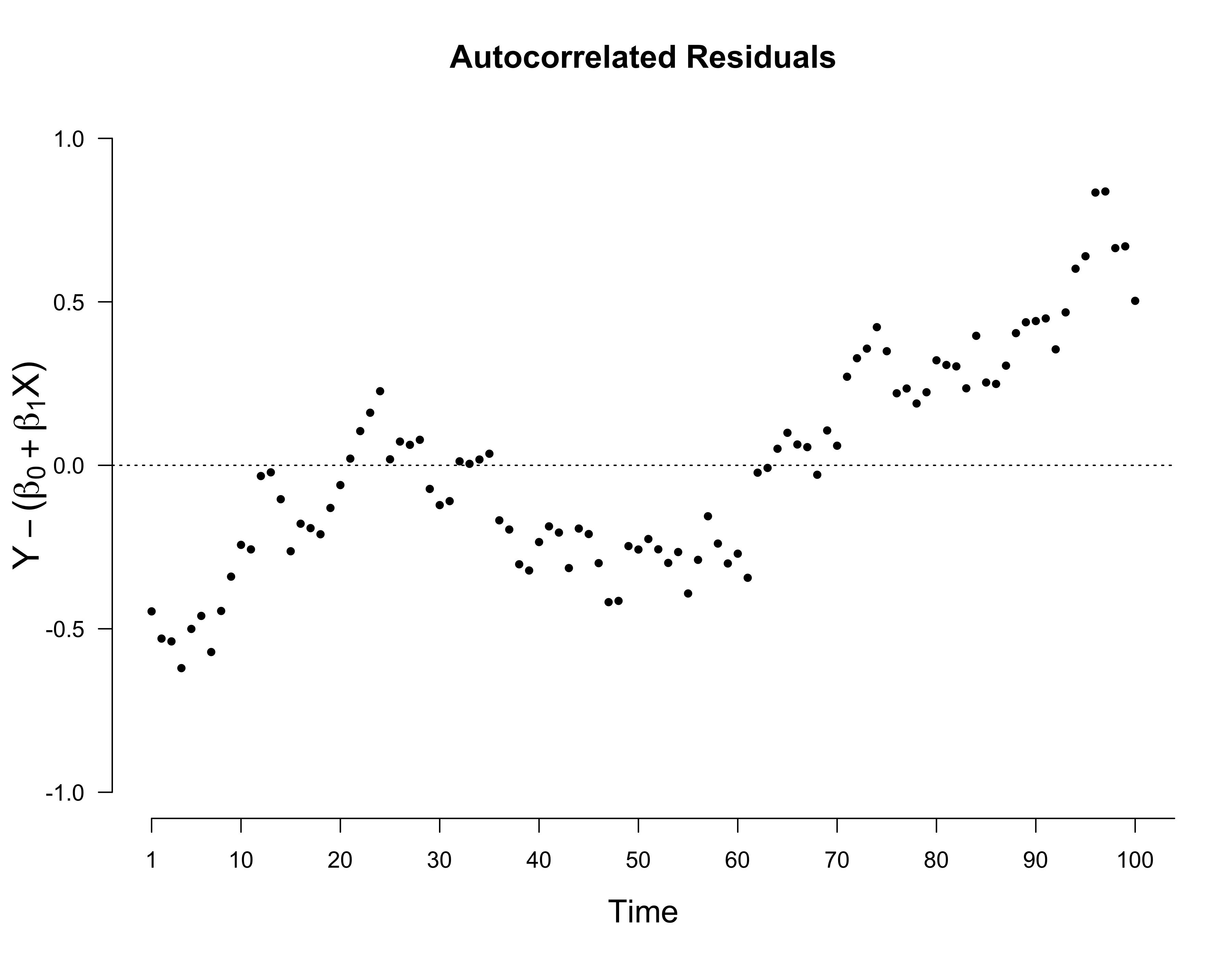
Similar as above, we can have an AR(1) process on the residuals:

and test whether $\delta = 0$. We can do so using the Durbin-Watson test, which yields:

car::durbinWatsonTest(m)

##  lag Autocorrelation D-W Statistic p-value
##    1       0.9357562    0.08623868       0
##  Alternative hypothesis: rho != 0

This indicates substantial autocorrelation, violating our modeling assumption of independent residuals. In the next section, we look at the deeper mathematical reasons for why we get such spurious correlation. In the Post Scriptum, we relax the constraint that $\phi = 1$ and look at how spurious correlation behaves for AR(1) processes.

Inconsistent estimation

The simulation results from the random walk simulations showed that the average (absolute) correlation stays roughly constant, while the test statistic increases with $n$. This indicates a problem with our estimator for the correlation. Because it is slightly easier to study, we focus on the regression parameter $\beta_1$ instead of the Pearson correlation. Recall that our regression estimate is

where $\bar{x}$ and $\bar{y}$ are the empirical means of the realizations $x_t$ and $y_t$ of the AR(1) processes $X_t$ and $Y_t$, respectively. The test statistic associated with the null hypothesis $\beta_1 = 0$ is

where $\hat{\sigma}$ is the estimated standard deviation of the error. In simple linear regression, the test statistic follows a t-distribution with $n - 2$ degrees of freedom (it takes two parameters to fit a straight line). In the case of independent random walks, however, the test statistic does not have a limiting distribution; in fact, as $n \rightarrow \infty$, the distribution of $t_{\text{statistic}}$ diverges (Phillips, 1986).

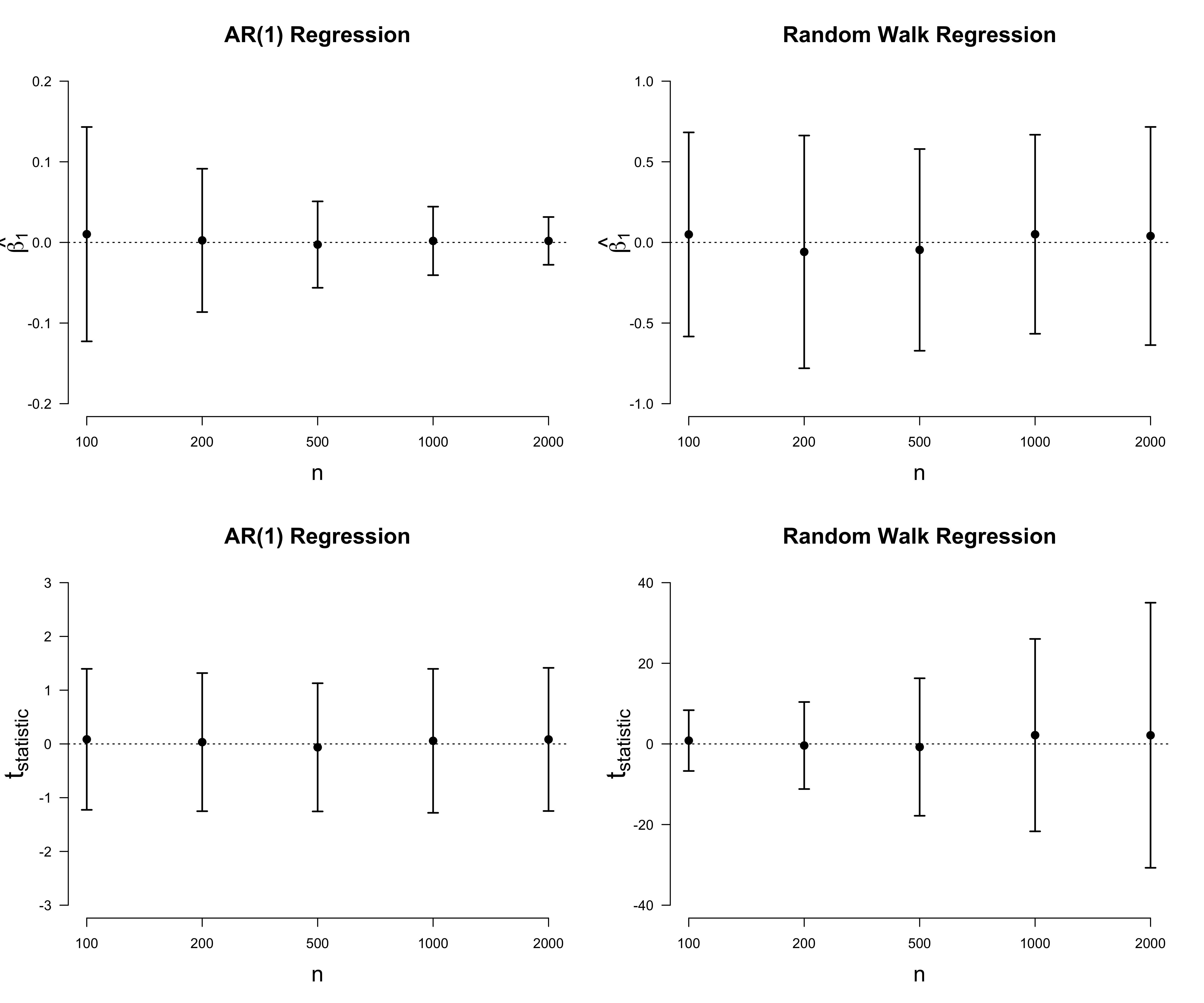
To get an intuition for this, we plot the bootstrapped sampling distributions for $\beta_1$ and $t_{\text{statistic}}$, both for the case of regressing one independent AR(1) process onto another, and for random walk regression.

regress_ar <- function(n, phi, sigma) {
  y <- simulate_ar(n, phi, sigma)
  x <- simulate_ar(n, phi, sigma)
  coef(summary(lm(y ~ x)))[2, c(1, 3)]
}
 
bootstrap_limit <- function(ns, phi, sigma, times = 200) {
  res <- matrix(NA, nrow = times * length(ns), ncol = 3)
  colnames(res) <- c('n', 'b1', 'tstat')
 
  ix <- 1
  for (n in ns) {
    for (i in seq(times)) {
      coefs <- regress_ar(n, phi, sigma)
      res[ix, ] <- c(n, coefs)
      ix <- ix + 1
    }
  }
 
  data.frame(res)
}
 
 
set.seed(1)
ns <- c(100, 200, 500, 1000, 2000)
res_ar <- bootstrap_limit(ns, .5, .1)
res_rw <- bootstrap_limit(ns,  1, .1)

The Figure below illustrates how things go wrong when regressing one independent random walk onto the other. In contrast to the estimate for the AR(1) regression, the estimate $\hat{\beta}_1$ does not decrease in the case of a random walk regression. Instead, it stays roughly within $[-0.75, 0.75]$ across all $n$. This shines further light on the initial simulation results that the average correlation stays roughly the same. Moreover, in contrast AR(1) regression for which the distribution of the test statistic does not change, the distribution of the test statistic for the random walk regression seems to diverge. This explains why we the proportion of false positives increases with $n$.

Rigorous arguments of the above statements can be found in Phillips (1986) and Hamilton (1994, pp. 577).³ The explanations feature some nice asympotic arguments which I would love go into in detail; however, I’m currently in Santa Fe for a summer school that has a very tightly packed programme. On that note: it is very, very cool. You should definitely apply next year! In addition to the stimulating lectures, wonderful people, and exciting projects, the surroundings are stunning⁴.

Conclusion

“Correlation does not imply causation” is a common response to apparently spurious correlation. The idea is that we observe spurious associations because we do not have the full causal picture, as in the example of storks and human babies. In this blog post, we have seen that spurious correlation can be due to solely statistical reasons. In particular, we have seen that two independent random walks can be highly correlated. This can be diagnosed by looking at the residuals, which will not be independent and identically distributed, but will show a pronounced autocorrelation.

The mathematical explanation for the spurious correlation is not trivial. Using simulations, we found that the estimate of $\beta_1$ does not converge to the true value in the case of regressing one independent random walk onto another. Moreover, the test statistic diverges, meaning that with increasing sample size we are almost certain to reject the null hypothesis of no association. The spurious correlation occurs because our estimate is not consistent, which is a purely statistical explanation that does not invoke causal reasoning.

I want to thank Toni Pichler and Andrea Bacilieri for helpful comments on this blog post.

Post Scriptum

Spurious correlation of AR(1) processes

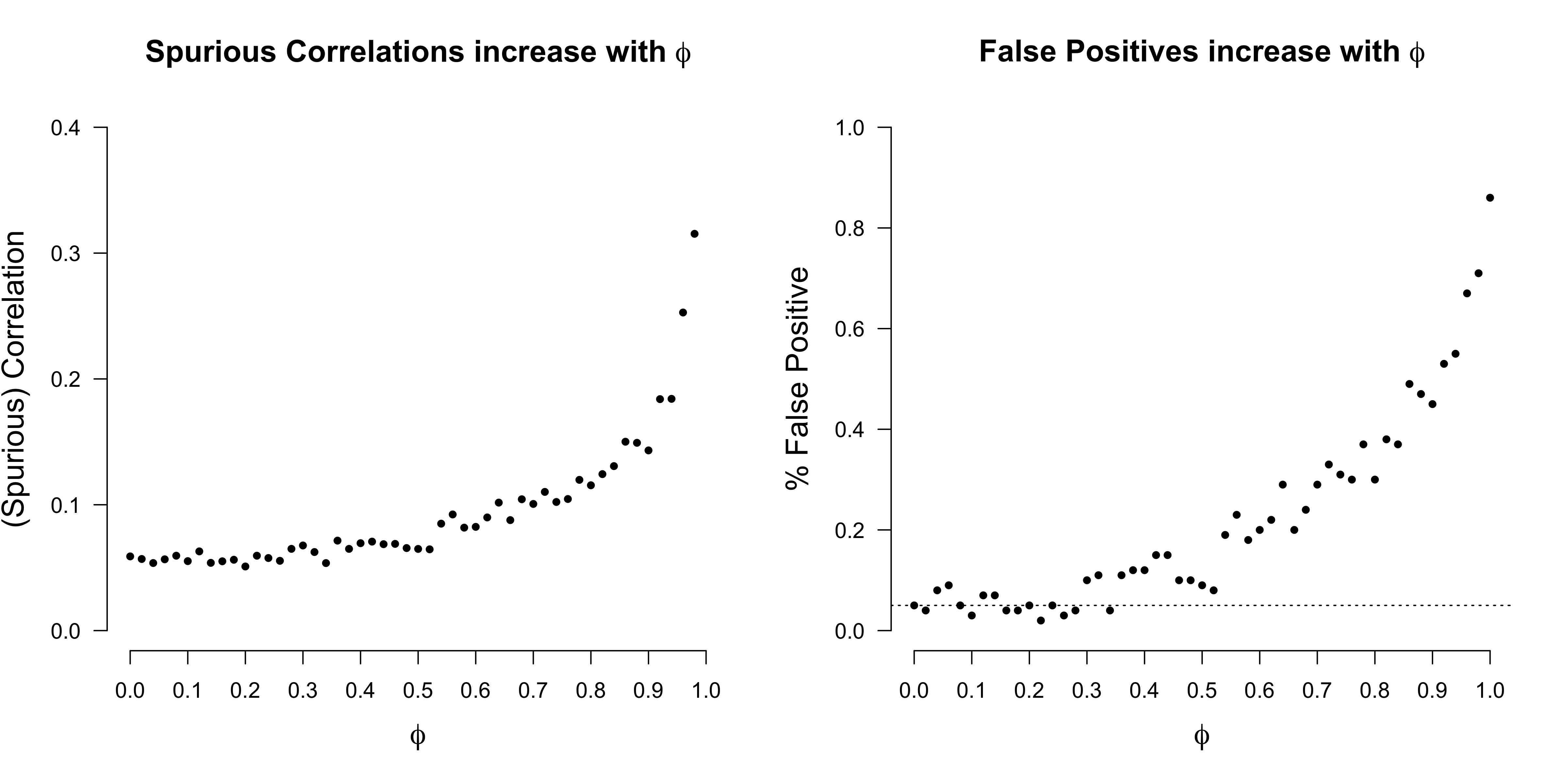
In the main text, we have looked at how the spurious correlation behaves for a random walk. Here, we study how the spurious correlation behaves as a function of $\phi \in [0, 1]$. We focus on sample sizes of $n = 200$, and adapt the simulation code from above.

set.seed(1)
 
n <- 200
times <- 100
phis <- seq(0, 1, .02)
comb <- expand.grid(times = seq(times), n = n, phis)
ncomb <- nrow(comb)
 
res <- matrix(NA, nrow = ncomb, ncol = 6)
colnames(res) <- c('ix', 'n', 'phi', 'cor', 'tstat', 'pval')
 
for (i in seq(ncomb)) {
  ix <- comb[i, 1]
  n <- comb[i, 2]
  phi <- comb[i, 3]
  
  test <- cor.test(simulate_ar(n, phi = phi), simulate_ar(n, phi = phi))
  res[i, ] <- c(ix, n, phi, test$estimate, test$statistic, test$p.value)
}
 
dat <- data.frame(res) %>% 
  group_by(phi) %>% 
  summarize(
    avg_abs_corr = mean(abs(cor)),
    avg_abs_tstat = mean(abs(tstat)),
    percent_sig = mean(pval < .05)
  )

The Figure below shows that the issue of spurious correlation gets progressively worse as the AR(1) process approaches a random walk (i.e., $\phi = 1$). While this is true, the regression estimate remains consistent.

References

• Granger, C. W., & Newbold, P. (1974). Spurious regressions in econometrics. Journal of Econometrics, 2(2), 111-120.
• Hamilton, J. D. (1994). Time Series Analysis. P. Princeton, US: Princeton University Press.
• Kuiper, R. M., & Ryan, O. (2018). Drawing conclusions from cross-lagged relationships: Re-considering the role of the time-interval. Structural Equation Modeling: A Multidisciplinary Journal, 25(5), 809-823.
• Phillips, P. C. (1986). Understanding spurious regressions in econometrics. Journal of Econometrics, 33(3), 311-340.
• Matthews, R. Storks deliver babies (p = 0.008) (2000). Teaching Statistics 22(2), 36–38.

Footnotes