Jekyll2024-09-27T17:23:38+00:00https://fabiandablander.com/feed.xmlFabian DablanderPostdoc Energy TransitionFabian DablanderDeep Learning for Tipping Points: Preprocessing Matters2022-05-10T16:15:00+00:002022-05-10T16:15:00+00:00https://fabiandablander.com/Deep-WarningThe text below is taken verbatim from Dablander & Bury (2022), which was published here.
Bury et al. (2021) present a powerful approach to anticipating tipping points based on deep learning that not only substantially outperforms traditional early warning indicators, but also classifies the type of bifurcation that may lie ahead. Their work is impressive, innovative, and an important step forward. However, deep learning methods are notorious for sometimes exhibiting unintended behavior, and we show that this is also the case for the method proposed by Bury et al. (2021).
We simulate $n = 500$ observations from an AR(1) process with lag-1 autocorrelation $\rho = 0.50$ and standard Gaussian noise term and apply the deep learning method. The left panel in Figure 1 shows the probability of a fold (red), Hopf (orange), transcritical (blue), and no (green) bifurcation, with solid lines indicating averages and shaded areas indicating standard deviations across 100 iterations. We find that the deep learning method suggests that the process is approaching a fold (or possibly a transcritical) bifurcation. The middle panel shows that detrending with a Gaussian filter with bandwidth $0.20$ improves performance, but substantial uncertainty remains. The right panel shows the results after detrending using a Lowess filter with span $0.20$, as performed by Bury et al. (2021).1 We find that the deep learning method is able to correctly classify the system as not approaching a bifurcation.
Figure 1. Deep learning classification for a stationary AR(1) process without detrending (left) and with detrending using a Gaussian (middle) and Lowess filter with bandwidth / span of $0.20$ (right). Solid lines show averages and shaded regions standard deviations over 100 iterations.
To further explore this behavior, we conducted the same analysis for a range of lag-1 autocorrelations $\rho \in [0, 0.05, \ldots, 0.95]$ and Lowess spans / Gaussian bandwidths $b \in [0.05, 0.075, \ldots, 0.50]$. The left panel in Figure 2 shows the probability of correctly classifying the time series as approaching no bifurcation after observing all $n = 500$ data points. Classification becomes more challenging as the lag-1 autocorrelation approaches 1. In general, the deep learning method performs better the smaller the Lowess span. Performance drops substantially, however, when using Gaussian filtering, as the right panel in Figure 2 shows.
Figure 2. Probability of correctly inferring that no bifurcation lies ahead after observing $n = 500$ data points from a stationary AR(1) process with a particular lag-1 autocorrelation that has been detrended with a particular Lowess span (left) or Gaussian bandwidth (right), averaged over 100 iterations.
Bury et al. (2021) trained the deep learning method only on time series that have been detrended using a Lowess filter with span $0.20$. While the authors showed that the method exhibits excellent performance in several empirical and model systems, we found that it did not extract features generic enough to classify stationary AR(1) processes that have not been detrended (or have been detrended using a Gaussian filter) as approaching no bifurcation. This sensitivity to different types of detrending suggests that the method may have learned features specific to a Lowess filter rather than (only) generic features of a system approaching a bifurcation.
Interestingly, detrending takes on a different purpose in this context: for traditional early warning indicators, adequate detrending helps avoid biased estimates (e.g., Dakos et al., 2012), while for the deep learning method developed by Bury et al. (2021) a particular type of detrending is necessary because all training examples were detrended using it. Both Bury et al. (2021) and Lapeyrolerie & Boettiger (2021) note that the training set would have to be expanded substantially to include richer dynamical behavior than fold, transcritical, and Hopf bifurcations. With this note, we suggest that other aspects of the training, including the preprocessing steps, also need careful consideration.
Footnotes
The Lowess span and Gaussian bandwidth are given as a proportion of the time series length; detrending was conducted using the ewstools Python package. ↩
]]>Fabian DablanderThe Barely Inhabitable Earth: Climate Impacts under Business as Usual2022-01-21T11:30:00+00:002022-01-21T11:30:00+00:00https://fabiandablander.com/Climate-Impacts
Climate change always felt like a distant, almost surreal threat to me. I learned about it in high school over ten years ago and thought: “This sounds pretty bad … But surely the people in power — the adults in the room — will manage to fix this and we can all just move on.” And so I grumbled on in the comfort and ignorance of my own life, focusing on individual consumption behaviour (no meat! no dairy! fewer flights!) as my way to contribute to the cause. As if isolated individual actions and hoping for the best would cut it.
What rattled me out of the comfort of my life was the COVID-19 pandemic. I realized that stability is not a given — things can change dramatically, quickly, and for the worse. I also realized that we cannot rely on the people in power to fix things. These realizations caused me to take another, more in-depth look at climate change. I started to read the scientific literature, attended talks and lectures, took courses on the topic, immersed myself in books, podcasts, and documentaries, invited climate scientists to speak at a colloquium I co-organized, and attended a conference on tipping points in the summer when Covid cases were low. You could safely say that I became obsessed with the topic.
Slowly, over weeks and months, I began to appreciate the gravity of the situation; it is, by all accounts, an emergency. Once you see it, you cannot unsee it anymore. But you have to force yourself to see it first. You have to pause and not — as I did for too many years — simply move on with your life. It is difficult. Engaging with this topic makes you feel sad, disappointed, angry, scared. Sometimes you feel hopeless. Sometimes you cry.
But there is hope. We are beginning to see the emergence of a truly global, massive climate movement, something it is exciting to be a part of — and something that is direly needed. The system transformations required to address the climate emergency are enormous, yet governments are either moving too slowly or in the wrong direction. To exert the necessary pressure to effect change, climate action has to move from something that a few others do to something that we all engage in. Each and every one of us has a role to play. It may sound grandiose, but this really is humanity’s decisive moment.
When I started to speak to friends, family, and colleagues about the climate emergency, I noticed that there is a general lack of awareness of how dire the situation is, and how bad it could still get if we continue on our current path. Although it is emotionally difficult to engage with the topic, any sober analysis of what needs to be done requires that we better understand the gravity of the situation. There is no way around it. In this blog post, I will therefore discuss the climate impacts that are already here, and how they would worsen under our current, business as usual trajectory, expanding on a recent workshop I gave.1
Lastly, a disclaimer: While I have discussed the facts and figures in these posts with climate scientists, all errors are mine. I am, as should be obvious, not speaking from a position of authority. Instead, I am speaking as a concerned citizen and a fellow traveller. Together, we can do this.
Let’s get on with it.
Business as usual
I was spending part of the pandemic lockdown isolated with my then girlfriend when I stumbled upon a book whose beginning shook me to the core. The book was The Future We Choose: Surviving the Climate Crisis by Christiana Figueres and Tom Rivett-Carnac, key architects of the Paris agreement. Here is an excerpt from its opening chapter describing a world in 2050 that is on a trajectory towards a 3°C temperature increase in 2100:
"The first thing that hits you is the thick air. In many places around the world, the air is hot, heavy, and depending on the day, clogged with particulate pollution. Your eyes often water. Your cough never seems to disappear."
"Extreme heat is on the rise. If you live in Paris, you endure summer temperatures that regularly rise to 44 degrees Celsius. Everyone stays inside, drinks water, and dreams of air-conditioning. You lie on your couch, a cold, wet towel over your face, and try to rest without dwelling on the poor farmers on the outskirts of town who, despite recurrent droughts and wildfires, are still trying to grow grapes, olives, or soy – luxuries for the rich, not for you."
"More moisture in the air and higher sea surface temperatures have caused a surge in extreme hurricanes and tropical storms. Recently, coastal cities in Bangladesh, Mexico, the United States, and elsewhere have suffered brutal infrastructure destruction and extreme flooding, killing many thousands and displacing millions. This happens with increasing frequency now. Every day, because of rising sea levels, some part of the world must evacuate to higher ground."
"Food production swings wildly from month to month, season to season, depending on where you live. More people are starving than ever before. [...] Disasters and wars rage, choking off trade routes. The tyranny of supply and demand is now unforgiving; because of its increasing scarcity, food can now be wildly expensive."
"Places such as central India are becoming increasingly challenging to inhabit. [...] Mass migrations to less hot rural areas are beset by a host of refugee problems, civil unrest, and bloodshed over water availability. [...] Even in some parts of the United States, there are fiery conflicts over water, battles between the rich who are willing to pay for as much water as they want and everyone else demanding equal access to the life-enabling resource."
"The demise of the human species is being discussed more and more. For many, the only uncertainty is how long we'll last, how many more generations will see the light of the day. Suicides are the most obvious manifestation of the prevailing despair, but there are other indications: a sense of bottomless loss, unbearable guilt, and fierce resentment at previous generations who didn't do what was necessary to ward off this unstoppable calamity."
This description might sound like hyperbole, using colourful language to evoke fear of what surely is an exceedingly unlikely dystopia. Digging into the details, I realized that it may not be. The latest projections suggest that continuing on our trajectory — business as usual — would lead to about 2.7°C of warming by 2100, with estimates ranging from 2°C to 3.6°C. This is a similar temperature increase as in the dystopia painted by Figueres and Rivett-Carnac. The key question, then, is about what climate impacts such a temperature increase would cause.
Climate impacts
Understanding the climate impacts happening already today and that our current emissions trajectory would further intensify is the core goal of this blog post.2 After discussing those, we will reflect on the fact that scientific models, while extremely powerful, are still only simplifications of the marvellous complexity of the real world — nasty surprises cannot be ruled out. And yet, fortunately, everything is still in our hands: the greatest uncertainty concerning climate impacts are our future emissions, which are entirely up to us. Dystopia is not a given. This is humanity’s decisive decade.
Dirty air
“A single death is a tragedy”, so the saying — widely attributed to Stalin — goes, while “a million deaths is a mere statistic.” But sometimes a statistic can still pull the rug out from under your feet. So it is with air pollution, which is estimated to kill between sevenandten million people every year already today — with heartbreaking stories from across the world — slashing average global life expectancy by more than two full years. Outdoor air pollution from the burning of fossil fuels is the main culprit. While estimates vary, the latest study puts the annual death toll from the pollution due to fossil fuels at 8.7 million globally — a death toll larger than that of smoking and malaria combined. Air pollution is also associated with a myriad of negative outcomes short of death, such as heart disease, cancer, asthma, and reduced cognitive performance. Regional impacts vary greatly, with Africa and South and East Asia taking the biggest hit.
Figure 1. Air pollution across the globe using data from IQiAir. For an explanation of their air quality index, see here.
The annual death toll due to air pollution is simply staggering. The latest estimates surpass the official death toll of COVID-19 so far, and are about half of all deaths that occurred in World War I. But while Figueres and Rivett-Carnac paint a picture of increasingly dirty air under business as usual, I am more confident that we will be able to reign in air pollution; just look at the recent progress in China.
Yet herein lies a cruel conundrum: aerosols from anthropogenic sources cool the Earth by about 0.50°C, as the latest assessment report (AR6) on the physical science basis from the IPCC notes. The major sources are sulphur dioxide, which has a cooling effect, and black carbon, which has a warming effect — both arise from the burning of fossil fuels. If we improve air quality and save millions of lives, the warming that aerosols mask will be set free. This warming can be counteracted by reductions in greenhouse gases such as ozone and methane, but only partly so. Combining changes in short-lived pollutants such as aerosols, ozone, and methane, the latest IPCC report finds that these changes could increase warming between 0.06°C and 0.35°C by 2040, depending on the scenario. The rate of warming in the next decades may thus increase sharply. This could intensify and hasten the climate impacts we turn to now.
Figure 2. Projected warming across the globe at a 2°C average increase over pre-industrial levels. From the IPCC's Interactive Atlas.
Extreme heat, combined with dangerous humidity that can impair the cooling effect of sweating and kill you, has more than doubled since the 1970s. If we do not curb emissions, vast swaths of the tropics — projected to be home to 50% of the global population by 2050 — may have regularly life-threatening wet-bulb temperatures. Indeed, a recent analysis found that at just 2°C of global warming, one billion people could experience wet-bulb temperatures exceeding workability thresholds. Barring strong adaptation efforts, huge areas of the globe may become uninhabitable.
Using climate projections with the SSP2-4.5 pathway3, which best resembles our current trajectory and would lead to about 2.7°C of warming by 2100, a recent report4 finds that half the global population will experience annual major heatwaves — defined as regional temperatures in the 99th percentile for at least four consecutive days — by 2050, with no region being spared. 44°C in Paris by 2050, as Figueres and Rivett-Carnac envision? No problem.
Storms and rising seas
Few extreme weather events embody the wrath of nature more powerfully than hurricanes. With 2021 being the third most active hurricane season to date — right behind 2020 and 2015 — frequent reminders of nature’s power abound. Indeed, hurricanes and tropical storms are becoming more intense and decay more slowly as temperature increase. Similarly, extreme flooding is also becoming more frequent. Warm air can hold more moisture — 7% more for every 1°C temperature rise — discharging it abruptly. Indeed, rainfall extremes have increased, with about a quarter of the most severe rainfall events in the last decade being attributable to climate change. Rich countries cannot think themselves in safety, with the intensity and scale of the 2021 flooding in Germany shocking climate scientists.
While tropical storms and extreme flooding focus minds on local destruction, it is rising sea levels that most vividly capture the planetary scale transformation a warming planet brings. The IPCC Special Report on the Ocean and Cryosphere notes that about 680 million people reside in low-lying coastal areas today, defined as being less than ten metres below sea level, a number that is projected to increase to over one billion by 2050. This exposes them directly to rising sea levels and coastal flooding. Since the 1900s, the sea has risen by about 0.20 metres, mostly due to thermal expansion, but with ice sheet and glacier mass loss being the dominant contributor since 2006.
Under our current emissions trajectory, sea levels are projected to rise between 0.66 and 1.33 metres by 2100. The melting of the ice sheets is a very slow process, however, with most of the sea level rise occurring after 2100. The current best estimate for the tipping point of the Greenland ice sheet — containing ice equivalent to 7.2 metres of sea level rise — is 1.5°C, with an uncertainty band from 0.80°C to 3°C. The West Antarctic Ice Sheet — containing ice equivalent to about 3.3 metres of sea level rise — could cross an irreversible tipping point between 1.5°C and 2°C of warming. With 3°C of warming, then, the total melting of these two ice sheets is certain, causing sea levels to eventually rise more than 10 metres, engulfing virtually all coastal regions and many major cities.
Figure 3. Latest sea level rise projections find much of Vietnam under water at high tide by 2050. From this article in The New York Times.
While the total melting of the Greenland ice sheet could take at least a millennium, regions situated in the Middle East and Asia such as Vietnam, Egypt, and Mumbai — comprising about 150 million people — are severely vulnerable to sea level rise already by 2050. With two key glaciers in the Antarctic — the Thwaites Glacier and the Pine Island Glacier — becoming destabilized more quickly than previously thought, sea level rise may further accelerate. Indeed, recent research suggests that our current pathway could speed up sea level rise by an order of magnitude by 2060.
Food and drink
If you are anything like me, then you probably know shockingly little about how our food gets produced. I once grew tomatoes, which was fun. For all other things, I visit my local supermarket. People like me are usually alienated from the land — even though we collectively use about half of it for agriculture. While all countries engage in agriculture, there are a number of major breadbaskets for the four major crops: maize (corn) is chiefly produced in the US (34%), China (23%), and Europe (10%); rice in China (28%), India (21%), and Indonesia (10%); soybeans in the US (34%), Brazil (30%), and Argentina (17%); and wheat in Europe (24%), China (13%), and India (13%).
For the first time in history, our own actions threaten our life support systems, food production in particular. Our current food system is already broken, with around 800 million experiencing chronic hunger, 3 billion unable to afford a healthy diet, 2 billion being overweight, a third of all food being wasted, and nearly all farm subsidies — 90% out of 540 billion yearly — causing harm. Our food system is still able to sustain us. It might cease to in the future.
You might come across the occasional scattered report about droughts impacting agriculture in your favourite newspaper. It is difficult to connect the dots when only passively consuming the news. But once you start looking for it, within minutes you find that agricultural droughts (that is, crop yield reductions or failures due to soil moisture deficits) are already experienced literally all over the world — from the United States, Canada, and Mexico to Chile, Brazil, and Argentina; from Madagascar, Kenya, and Angola to Afghanistan, Iran, and Jordan; from Europe to China and all the way down to Australia. Climate impacts on agriculture are here. But they could become much worse.
Using the SSP2-4.5 pathway, which would lead to about 2.7°C of warming by 2100, a recent report finds that, assuming that the global cropland remains constant at 14.7 million km$^2$, 40% of this area will be exposed to severe drought for three months or more each year by 2050. This is compared to just 9% between 1981 and 2010. Europe, which has the second-largest cropland area — 20% of the global total — would experience such severe droughts in nearly half the cropland area. Southern Europe will be hit harder than the North, likely further driving a wedge within the European Union. Africa and North America, which represent 14% and 15% of the global cropland, are projected to suffer severe drought on 44% and 38% of the cropland, respectively.
Figure 4. Proportion of cropland projected to be exposed to severe drought every year by 2050. Adapted from here.
There are important benefits for plants in a warming world, however. An increase in CO$_2$ in the atmosphere can markedly increase global photosynthesis, and has done so by about 12% between 1981 and 2020. This effect known as CO$_2$ fertilization. Increased CO$_2$ levels are known to increase the yields of C$_3$ crops, which include wheat and rice, if ample nutrients and water are available. They do not significantly increase the yields of C$_4$ crops, however, which include maize. The difference between these two types of crops is that C$_4$ crops have evolved a mechanism to minimize photorespiration, and can thus survive well in hot, sunny environments. CO$_2$ fertilization can further decrease crop evotranspiration, the process in which water moves from the soil into the atmosphere. This improves the water-use efficiency for crops, which makes them more resistant to drought.
A major recent study, using the latest generation of crop and climate models, projects that the average crop productivity — a measure of crop yield — by the end of the century could decline strongly for maize (ranging from -6.4% to -24.1%); increase markedly for wheat (+8.8% to +17.5%); stay roughly the same for soybeans (+2% to -2.1%); and increase slightly for rice (+3.4% to +1.7%). These ranges indicate a best-case and a worst-case climate mitigation scenario, respectively. The authors further note that climate impacts are projected to arrive earlier than in the previous generation of models.
These averages hide important regional differences, however. Tropical and subtropical regions, where increasing temperatures have the largest impacts, will see large declines in maize. In contrast, in higher latitudes where wheat is generally grown, warming will increase gains. We will explore this familiar injustice — countries least responsible for climate change will suffer the harshest consequences — in the second part of this series in more depth. For now, note that this shift of agricultural zones has the potential to cause severe disruptions of the food system and requires strong adaptation efforts.
Importantly, these insights and estimates are derived from models that by their very nature abstract away complexity and do not include all relevant factors; they may thus give us an overly optimistic picture of what lies ahead. The Herculean effort mentioned above, for instance, does not incorporate insect pests, which could depress global yield substantially, although the details about the response of individual species are complex. Similarly, the study does not incorporate the fact that increased CO$_2$ levels can significantly decrease the nutritional value of crops, nor does it model water scarcity.
Major breadbaskets are projected to experience water scarcity, which could impede irrigation. Under such circumstances, a recent study finds that the probability of annual global crop failures, defined as a 10% decline in yield, will nearly triple for maize (reaching 30%) and about double for wheat and soybean (reaching 20%) already by 2030. Such declines would cause significant spikes in food prices in rich countries — leading to social unrest — and mass starvation and famine in poorer countries. Overall, the climate impacts on agriculture are very concerning, especially given the fact that we will need to produce about 50% more food to feed an additional two billion mouths by 2050.
Water is key not only for plant, but also for human life. Climate change will exacerbate hydrological droughts (that is, water shortages in streams or storages such as lakes), leading to decreased water availability. On the SSP2-4.5 pathway, the global population experiencing a hydrological drought of at least six months would be nearly double the historical average by 2040, reaching almost 700 million souls.
The severity of these droughts would be at least as bad as the 1934 wave of the Dust Bowl drought in the US, known as the “drought of record”. No region will be spared, but East and South Asia, with 125 and 105 million people being impacted, respectively, and Africa, with 152 million people being impacted, will see the most severe consequences by 2040. Europe will see the greatest increase in droughts in percentage terms (120%) compared to a scenario with no additional climate change.
Internal displacement and migration
I have had the enormous privilege to live in a number of wonderful European cities. After a period in which I completed part of my studies, I moved from one city to the next, full of melancholy about leaving but also excited to explore new opportunities. I always moved by choice. Millions of people do not; it is difficult to truly grasp their pain and trauma.
The United Nations Refugee Agency notes that, by the end of June 2021, the number of people displaced in their own country has risen to nearly 50.9 million people. The majority of internal displacement is already caused by weather-related disasters, amounting to about 30 million people in 2020. China (5.1 million), The Philippines (4.4m), Bangladesh (4.4m), India (3.9m), and the United States (1.7m) were hit the hardest. While many weather-related internal displacements are temporary, by the end of 2020 at least 7 million people globally were persistently uprooted. It is of course difficult to attribute any single extreme weather event to climate change, but we have seen above how climate change has played already an important role in increasing the frequency and intensity of such events. And it is getting worse.
Figure 5. Global internal displacements in 2020 due to conflict (orange) and weather-related disasters (blue). From here.
The situation can also become so dire that people are forced to leave their home country, becoming refugees. The United Nations Refugee Agency estimated that the number of global refugees has surpassed 20.8 million by mid-2021, with the majority coming from Syria (6.8 million), Venezuela (4.1m), Afghanistan (2.6m), South Sudan (2.3m), and Myanmar (1.1m). Migration never has a single cause, arising instead from an interconnected web of social, economic, political, and climatic factors. Under our current business as usual trajectory, however, migration could become much, much worse.
As we have seen above, increasingly uninhabitable zones — be it due to extreme heat, sea level rise, famine, or lack of water — will inevitably force people to move. While quantifying environmental migration is challenging, some work exists that hints at the scale of the climate migration that lies ahead. For one, humans have evolved in a surprisingly small climate niche, with mean annual temperatures of around 13°C. A nightmarish emission scenario would result in up to 3.5 billion people living outside this climate niche by 2100. This emissions scenario, which would lead to nearly 5°C of warming by 2100, is fortunately unlikely. Yet even limiting warming to 2°C would push 1.5 billion people — nearly 20% of humanity — outside the climate niche. This does not, of course, directly translate to migration, which, among other things, depends crucially on adaptation options. But these results indicate the scale of the historic transformation that is underway.
In a recent report, the World Bank estimates that up to 212 million people could be displaced within their countries by 2050. Another recent report puts the number of people that could be displaced by 2050 at 1.2 billion.
Whatever the actual numbers, recall the Syrian civil war, to which a drought amplified by climate change contributed and which lead to about 6.8 million Syrians leaving their home country. The conflict led to a wave of migrants which led to a steep rise in right-wing politics and parties in Europe. Imagine increasing this number by a one or even two orders of magnitude. Our already weakened political system would not stand this pressure. Ecofascism, already on the rise, might become the dominant sentiment. Social cohesion might erode.
While being a major threat itself, climate change is also a threat multiplier. Whatever problem arises, climate change will likely exacerbate it. This is how the Pentagon, which has an enormous carbon footprint and which is busy making preparations, viewsthe issue. A warmer climate or increased precipitation is linked to increasing conflict. Conflict is also enhanced by climate-related disasters, especially in ethnically fractured countries. Naturally, conflicts over resourcesbecome more likely as food and water insecurity increase. Tensions between nuclear armed states, such as Pakistan and India, both strongly exposed to climate impacts, might escalate as the situation worsens.
In summary, continuing on our current trajectory would lead to extreme heat and heatwaves of increased duration and frequency that would impact billions of people; more hurricanes, tropical storms, and extreme flooding; increased sea level rise that would uproot hundreds of millions of people; increased agricultural and hydrological droughts leading to crop failures, famine, and water stress; mass migration and conflict over resources. It is with this bleak vision of our future, one that we are currently hurdling towards, that Figueres and Rivett-Carnac imagine, by 2050, that the “demise of the human species is being discussed more and more.”
The map is not the territory
The previous section makes it abundantly clear that there is ample reason to act, swiftly and with resolve, if we wish to avoid the worst outcomes. But it makes sense to step back for a second and reflect on how we make sense of this moment. Climate scientists use very sophisticated models to better understand the world and predict how it might change under different circumstances. Modelling is an extremely powerful approach, and science, more broadly, has been an invaluable tool for humanity; it is by far the best thing we have to make sense of a changing world.
But while the scientific consensus is absolutely clear on the emergency situation we are in — it is “code red for humanity” — our understanding of the climate and the Earth system is not perfect. Climate models have done a reasonably good job at predicting future warming, but they may well have underestimated the extent of the climate impacts — as evidenced by the surprisingly severe floods and a wobbly jet stream causing the freakish heat dome last summer that shattered temperature records by up to nine degrees Celsius.
On the same token, advances in research usually suggest worsening impacts, as we have seen above with regards to air pollution, extreme heat, sea level rise, and agriculture. This is frightening, as it suggests that the already hellish impacts outlined above might turn out to be worse — and may happen sooner — should we choose to continue with business as usual. One prominent area of research hints at this possibility.
Tipping elements
The projections sketched above — and climate models more generally — tend to not capture tipping elements well. Tipping elements are large-scale components of the Earth system that, once a critical threshold is passed, can transition into an undesirable state, a transition that is generally irreversible on human time scales. These are high impact events which can wreak havoc on regional or even global scales.
The Greenland ice sheet, as mentioned above, is one such tipping element. Once a critical temperature threshold is crossed, runaway melting is set in process that is extremely hard to reverse. While the full melting of Greenland would take millennia, other tipping elements can wreak havoc on much shorter time scales. The Amazon rainforest is one such example. The mechanism is complicated and debated, but once a critical temperature threshold — combined with a deforestation threshold — is crossed, parts of the Amazon cannot efficiently generate their own rainfall anymore. This could lead them to tip into a savannah, potentially releasing an enormous amount of carbon dioxide into the atmosphere.
Figure 6. Map of selected tipping elements, adapted from Lenton et al. (2019).
Another tipping element is the Atlantic Meridional Overturning Circulation (AMOC), a system of ocean currents in the Atlantic Ocean of which the Gulf Stream — first sketched by Benjamin Franklin — is a part of. The AMOC transports warm, salty water from the tropics to Europe and beyond. There it cools and sinks, returning the cold water to the tropics. This heat exchange warms Europe and cools the tropics. As more freshwater feds into other North Atlantic — due to increased rainfall and increased melting of the Greenland ice sheet — it makes the water less salty, preventing it from sinking into the depths of the ocean, thereby slowing down the AMOC.
Permafrost thawing is another tipping element in the climate system that is not well represented in models. Permafrost is ground that stays frozen for at least two consecutive years, containing large amounts of dead plants, animals, and microbes. It underlies most of the Arctic, covering about 15% of the Northern Hemisphere, and holds about 1,600 billion tonnes of carbon dioxide, which is more than twice the amount we have in the atmosphere today.
When permafrost thaws it unfreezes microbes which decompose organic material, releasing methane and carbon dioxide. While the most recent IPCC report expresses high confidence that warming will lead to carbon dioxide release from the thawing of permafrost, it expresses low confidence in the size and timing of the emissions. Nonlinear processes such as abrupt thawing events, wildfires, and the fact that increased plant growth can speed up microbial production are not incorporated into models, but could greatly amplify permafrost thawing. In fact, some researchers argue that our lack of understanding is so grave as to question the size of our remaining carbon budgets.
Interconnections and the forgotten limit
Importantly, these tipping elements are interconnected and can potentially lead to tipping cascades. It may thus not be possible to ‘safely’ land at, say, 2°C — instead, tipping elements might further amplify global heating. Using a simplified modelling approach, recent research found that an increase in the melting of Greenland can cause the AMOC to slow down, which leads to less efficient cooling of the tropics which can increase the chances of (parts of) the Amazon tipping.
Equally concerning, scientists discovered that systems can tip when a critical rate of warming is exceeded even when a critical threshold is not. As an example of such “rate-induced tipping”, researchers recently found that the AMOC may tip when a critical rate of ice melt is exceeded even when a critical threshold is not.
Our climate targets, while mentioning critical rates in the early years, now only speak of thresholds such as 1.5 and 2°C, ignoring critical rates completely. This may be a huge blind spot, especially considering that the rate of warming is unprecedented in at least the last 24,000 years. At the same time, the IPCC has continuously revised their risk assessment concerning tipping elements upwards: while the third assessment report (AR3) in 2001 has classified the risk of tipping points as ‘undetectable’ with even a 3°C rise, the IPCC Special Report released in 2018 quantifies the risk as ‘moderate’ to ‘high’ already at 2°C. The most recent assessment of tipping points reinforces the extremely high risk associated with our current trajectory.
Precaution be damned
The above shows that uncertainty tends not to be our friend, and that unmodelled factors substantially increase the risk of our current emissions trajectory. Earth’s climate is extremely complex, with a delicate balance in place across its multiple interconnected systems. Include the social system, and uncertainty goes through the roof. A severe drought in the Middle East helped create the conditions for the Arab Spring, the ensuing Syrian civil war and a refugee crisis that lead to a rise in right-wing populism that further derails action on climate.
That’s a nice story, maybe even a plausible one. But actually foreseeing these network effects is next to impossible — life is too complicated, irregularities abound. Cascading climate impacts, which are impossible to model adequately let alone predict, could plunge the world into chaos. Once things begin to crumble and crack, the disintegration of society may well unfold rather quickly. Because of our lack of understanding of key Earth system elements and their interactions with the social domain, the extent and timing of the hellish consequences our current pathway pushes us towards may be profound underestimates of what could lie ahead.
At no point in history have we ever violated the precautionary principle with such ferocity and dogged determination as we do today. With the current atmospheric concentration of CO$_2$ at 417ppm, something last seen three million years ago, we are already exceeding the planetary boundary of 350ppm that is considered “safe” by Earth system scientists. The consequences of this transgression are becoming increasingly apparent. But they could, as we have seen, become much worse. We are in an emergency. We have no time to lose.
Choices
In the year 2050, I will be 57 years old. My kids, should I decide to have any, might just be reaching university age. Your situation might be similar. Maybe you already have kids, and are wondering about their future. Are we really going to let this happen? Do we really want to spend our old age living through the collapse of civilization, a sense of bottomless loss and unbearable guilt in our hearts, the fate of our young children sealed?
I know I don’t want this. And you probably don’t want this either. And so here we are, at a precipice. At a historic moment in our individual lives and our species at large. We have been given a distressing choice, but a choice nonetheless: do we stand by as this enormous catastrophe unfolds, or do we rise up and do everything we can to try to avert it — to rattle ourselves out of the paralyzing comfort of our current lives and rage, rage against the dying of the light?
In The Future We Choose: Surviving the Climate Crisis, Figueres and Rivett-Carnac sketch another future — one where energy is derived from renewable sources, trees cool cities, buildings produce their own electricity, high-speed electric railways have replaced the vast majority of domestic flights, and industrialized farming has given way to regenerative agriculture. This world is still possible. But it is getting late.
There is a scene in The Lord of the Rings I think about frequently in the context of the climate emergency. “I wish the Ring had never come to me. I wish none of this had happened”, says Frodo, to which Gandalf replies: “So do all who live to see such times, but that is not for them to decide. All we have to decide is what to do with the time that is given to us.”
The people in power have squandered the time that was given to them. Key decades have passed in which we could have made minor adjustments to business as usual to prevent climate breakdown. Instead, emissions have soared. And so today we are cornered — forced to take decisive action if we wish to hold on to the hopes and the dreams we have for our lives and our loved ones.
We cannot change the past. But we can, as Gandalf reminds us, still change the future.
The title of this blog post is inspired by the 2017 piece The Uninhabitable Earth by David Wallace-Wells. Wallace-Wells used the worst-case climate projections — which would lead to nearly 5°C of warming by 2100 — and vividly described the hellish consequences this could unleash. Such a scenario is considered unlikely today. Instead, I focus on our current emissions trajectory, which would lead to about 2.7°C of warming by 2100 (with some caveats applied that we will explore later in the post). That world might not be uninhabitable. But it would still look nothing like our world looks today. ↩
In his wide-ranging new book The Nutmeg’s Curse, Amitav Ghosh notes that, in the West, the climate crisis is generally treated as an isolated issue and as something that lies in the future. In contrast, Ghosh notes, people from the Global South, who are at the frontlines and already suffer severely from climate impacts, generally view the climate crisis as happening right here, right now; as being interconnected with many other crises; and as a familiar injustice, a continuation of colonialism and imperialism. I will explore this injustice in greater depth and discuss the climate crisis as one of several interlinked crises in the second post of this series. Climate impacts are indeed already experienced everywhere. But, at least for me, there is nothing that focusses my mind and compels me to act more strongly than knowing just how dramatically our current trajectory could upend the world as we know it. Hence this blog post. ↩
Since one cannot predict the extent of future emissions and how society develops, the climate modelling community relies on scenarios or narratives of the future. There exist five different so-called Shared Socioeconomic Pathways (SSPs), which can be combined with various climate mitigation scenarios. The latter are distinguished by the extent of the radiative forcing — the difference between incoming and outgoing power in Watts per square metre — by 2100. SSP2-4.5 combines the SSP2 scenario — called “middle of the road”, in which past societal trends continue⭑ — with a mitigation scenario that limits radiative forcing to 4.5 W/m$^2$ by 2100, resulting in a median of about 2.7°C of global heating by 2100. In this scenario, we would reach 1.5°C in 2032 (median; range: 2026 - 2042) and 2°C in 2052 (median; range 2038 - 2072). I quote median estimates throughout, although one would be well advised to look at the whole distribution and — given that uncertainty tends not to be our friend — revise estimates accordingly. For an excellent introduction to the SSPs, see this post over at CarbonBrief, the best source of information on climate. ⭑A caveat: The SSPs were developed in a world before Brexit, before Trump, before the resurgent nationalism we see around the world today. Indeed, our current trajectory may well resemble SSP3 — called “regional rivalry” — more closely than SSP2. International collaboration on climate is more difficult in SSP3, leading to higher mitigation and adaptation challenges and generally worse outcomes. Life can get ahead of science very quickly these days it seems. ↩
The Chatham House report I refer to summarises the results regarding the SSP2-4.5 scenario detailed in Arnell et al. (2019). This research uses projections from the Coupled Model Intercomparison Project 5 (CMIP5), while the IPCC AR6 by Working Group I (on the physical science basis) draws on projections from CMIP6. In other words, the results I mention based on the Chatham House report do not use the latest generation of climate models. Given that climate impacts generally turn out to be worse and / or happen sooner than anticipated, I do not think that using the previous generation of models overestimates the risks; if anything, it might underestimate it. For a short summary of what the latest IPCC report by Working Group I has to say about extreme weather events and climate risks, see here. Also be sure to keep an eye out for the report by Working Group II (on impacts, adaptation, and vulnerability), which will go into these matters in much greater depth; it is scheduled to be released at the end of February 2022. ↩
The IPCC distinguishes betweenconfidence and likelihood. Confidence is “a qualitative measure of the validity of a finding, based on the type, amount, quality and consistency of evidence […] and the degree of agreement.” Likelihood, on the other hand, is “a quantitative measure of uncertainty in a finding, expressed probabilistically”, based on “statistical analysis of observations or model results, or both, and expert judgement by the author team or from a formal quantitative survey of expert views, or both.” Only if there is sufficient confidence (and a probabilistic assessment exists) does the IPCC attach probabilities to outcomes. ↩
The situation is dire, but if we join forces and engage in collective action we can save what still can be saved and indeed create a happier, healthier, fairer, and more sustainable society. If you want to get active, I suggest reading this excellent three-part series on climate action by Julia Steinberger and finding a climate action group in your local area. I also touch on climate action in a recent workshop I gave. Thanks for reading, and a warm welcome! Together, we can do this. ↩
]]>Fabian DablanderUnderstanding and preventing climate breakdown2022-01-06T14:30:00+00:002022-01-06T14:30:00+00:00https://fabiandablander.com/Climate-Workshop
The unusually stable climate of the past 10,000 years has enabled agriculture and civilization. And without further intervention, at least another 10,000 years of stability would have ensued. Yet starting in the 1950s, in what has been dubbed The Great Acceleration, humans dramatically grew their population and their economies, becoming a planetary-scale geological force that continues to exert enormous pressure on the Earth system. The consequences of this are becoming increasingly apparent. But they could become much worse.
There is, however, still a chance to avert the worst and, in the process, create a better world than we have today. But the challenge is monumental, the necessary system transformations enormous. To be on track to limit warming to 1.5°C requires that we cut global carbon emissions in half by 2030. Yet the people in power have failed, and continue to fail, to enact changes commensurate with the scale and urgency of the climate emergency. We cannot remain inert and just hope for the best.
Instead, we need to build the largest, most inclusive social movement in history and make it be heard that we do not stand for the continued destruction of the natural world. Climate action has to move from something that others do to something that we all engage in. Each and everyone of us has a role to play — this is humanity’s decisive decade.
I recently explored these themes – future climate impacts, our failure to bend the emissions curve so far, and what we can do today – with the CorrelAid Netherlands community in a workshop on the climate emergency and climate action. After an introductory talk of about 60 minutes, situating ourselves in this unfolding drama, we tried to find policies that limit warming to well below 2°C and ideally to 1.5°C in an equitable and just manner using En-ROADS, an interactive climate simulator.
What if we planted a trillion trees? Massively scaled up nuclear energy? Kept fossil fuels in the ground? All turned vegan? Introduced a world-wide carbon tax? These are some of the questions we addressed. Ultimately, we ended up with a scenario that limits warming to 1.8°C. Not too bad.
The workshop was intense. It lasted more than two hours and thirty minutes, with 45 people attending. We had wide-ranging conversations, from the basics of climate science to the finer details of mitigation modelling; from individual responsibility to considerations of justice; from structures of power to social movements and effective action. I felt that people came away with a better understanding of the many facets of the climate emergency and a renewed sense of, if not hope, then of the necessity to take action. Hope is what we create through action.
We unfortunately messed up the recording of the event, so I recorded it again without an audience. This means that the interactive part is not included. However, I do provide a short rundown of the En-ROADS simulator. If you think that such an interactive workshop could be valuable to you and your community, do not hesitate to reach out — I am always up for discussing climate and climate action.
A version of this blog post first appeared on the blog of CorrelAid Netherlands, an initiative that connects data scientists with organizations that advance the social good. If you want to learn more about the climate emergency and could benefit from an overview of resources, you might find this selection helpful.
]]>Fabian DablanderSimulation-based Science: Breaking Boundaries2021-07-18T10:30:00+00:002021-07-18T10:30:00+00:00https://fabiandablander.com/Simulation-based-ScienceSimulations are integral to many scientific disciplines and inquiries. I was therefore delighted when Mike Lees asked me to organize — together with Eric Dignum, Alex Gabel, Christian Spieker, Anna Keuchenius, and Vitor Vasconcelos — the Simulation-based Science colloquium for the summer semester 2021. The colloquium is usually hosted at the Institute for Advanced Study, but it is on Zoom that we met weekly. We split the task of inviting speakers amongst ourselves, and created what I think is an impressive line-up of 18 speakers with a wide range of backgrounds. All talks except the first one have been recorded and are available on YouTube (see here for a short description of all talks).
I am at a psychology department — the Department of Psychological Methods at the University of Amsterdam — and one reason why I was asked to help organize the colloquium might have been to find good speakers from psychology or closely related fields.
Psychology?
I did little to advance this goal. The closest I got to was inviting my colleague Maarten van den Ende to briefly speak about his excellent work on modelling of psychological and social dynamics of urban mental health conditions. To facilitate this type of work, Mathijs Maijer and Maarten have developed an impressive Python package that you may find useful for your own projects. While Maarten pursues psychological topics, he takes a distinctly interdisciplinary approach.
If gracious, you might say that inviting Paul Smaldino counts, who is well-known in psychology and who repeatedly and forcefully articulated the usefulness of formal modelling (e.g., Smaldino, 2017, 2019). A core problem of psychology is its curriculum, and Smaldino (2020) lays out the importance of increasing interdisciplinarity, technical skill, and philosophical scrutiny. Having stopped studying psychology after my undergraduate degree because of a lack of mathematical training and the fact that lectures and published psychological papers were often just a series of non sequiturs, it is good to see these issues articulated so well in print.
In his talk, Paul eschewed distinctly psychological content, however, and instead talked about his recent work on how interdisciplinarity can spread better methods (Smaldino & O’Connor, 2020). (Paul also showed an excerpt from what is probably my favourite Noam Chomsky interview).
The argument is as simple as it is compelling: having people from other disciplines take a critical look at the work a particular field is doing may help that field discover more quickly whether it is stuck in a local optimum. Local optimum may be too charible a phrase, however. Paul mentions the case of “magnitude-based inference” in sports science, a statistical method which was not described in equations but distributed as an Excel spreadsheet, wrecking havoc after its introduction.
For disciplines (overly) focused on empirical work such as psychology, statisticians are a natural outside group to assess the sensibilities of the field’s inferences. From a bigger picture perspective, however, conversations with anthropologists, philosophers, physicists, economists, ecologists, etc. may be even more insightful. They certainly would be more fun. Unfortunately, few places exist exist where such mingling is encouraged.
Automation
The first speaker I invited was Maria del Rio-Chanona, who gave a fantastic talk about her work on occupational mobility and automation (del Rio Chanona et al., 2021). At the core of this work is an occupational mobility network, a directed and weighted network whose nodes are occupations and whose weights give the probability that a worker transitions between occupations (and which is calibrated using US data). Running an agent-based model on this network and using estimates of the potential for automation of different occupations, Maria and her colleagues explored the effect of automation shocks. These shocks reallocate labour in the economy, increasing demand for it in occupations with a low potential for automation and decreasing demand for it in occupations with a high potential for automation.
A key finding is that the impacts on workers do not only depend on the automatability of their current occupation, but also on the automatability of occupations they could transition into. For example, ‘statistical technicians’ have a much higher probability of being automated than childcare workers, yet the prospects of long-term unemployment are worse for the latter. The authors note that this is because it is relatively easy for statistical technicians to transfer into occupations that increase in demand. On the flipside, it is relatively easy for workers in occupations that are susceptible to automation to transfer into childcare work, increasing those workers’ supply relative to their demand. As this example shows, and as Maria and colleagues argue more generally, network effects are more likely to hurt workers in low-income occupations, while workers in high-income occupations are more likely to benefit.
Maria and her colleagues also studied supply and demand shocks brought about by COVID-19 in a paper that I found very illuminating as the pandemic got going in early 2020 (del Rio Chanona et al., 2020). Their work nicely visualizes the extent to which different occupations might be affected, finding that — as in the case of automation — workers in low-income occupations are again more vulnerable than workers in high-income occupations.
Agent-based models are a key tool in complexity economics (Farmer & Foley, 2009; Arthur, 2021), a field that aims to provide a more realistic perspective on the economy — and, as far as my experience goes, also makes for very enjoyable papers. Incidentally, when I asked Maria why her paper on automation was not published in an economics journal, she was a bit taken aback (and rightfully so), saying that she considers this work interdisciplinary — an econ journal just would not do.
Tipping points
I then invited Jonathan Donges, who gave a truly wide-ranging and impressive talk, summarizing the work he did and is doing together with colleagues at the Potsdam Institute for Climate Impact Research on tipping points in the climate system and in the social sphere.
Jonathan noted that there exist considerable uncertainties in climate tipping elements pertaining to their exact thresholds and the strength and sign of their interactions. At the same time, tipping elements are not fully represented in state-of-the-art Earth system models, which are also too slow to run large-scale ensemble simulations with that are required for a risk analysis under large uncertainties. This motivates a simplified modelling approach that captures the essence of tipping elements and their interactions, which Jonathan and others found in the coupling of cusp catastrophes on complex networks (e.g., Klose et al., 2020; Krönke et al., 2020). Using this approach, Wunderling et al. (2021) studied four tipping elements and found that interactions between them tend to destabilize the system, implying significant risk of tipping cascades already at 2°C.
Tipping points are usually defined in terms of critical thresholds: going above a critical level of, say, temperature causes the system to transition into an alternative stable state. However, systems can also tip when a critical rate is exceeded (for an excellent introduction, see Siteur et al. 2016). I asked Jonathan whether this type of tipping is something that needs more attention since the rate of temperature increase — and not only its absolute level — is also extraordinary, while at the same time the Paris climate agreement and other policy frameworks only define critical thresholds. Jonathan replied that the lack of consideration of critical rates is indeed problematic, and that there is more evidence accumulating suggesting that rate-induced tipping can occur in climate tipping elements (e.g., Lohmann & Ditlevsen, 2021). He also mentioned, anecdotally, that John Schellnhuber — founding director of PIK — proposed to consider both critical thresholds as well as critical rates already in the 1990s; however, rates were thrown out because it was considered too complicated for politicians. During a similar discussion, Schellnhuber confirmed this anecdote at an all-star panel on tipping points. (I noticed later that this is actually also described in Schellnhuber, Rahmstorf, & Winkelmann, 2016).
As Jonathan pointed out, while we have some understanding of the tipping dynamics in the climate system, our understanding of tipping dynamics in the social domain is much more limited. For example, it is relatively straightforward to map the important drivers for climate tipping points on global temperature increase; but it is basically impossible to map dramatic changes in, say, public opinion on any single driver. Winkelmann, Donges, et al. (2020) discuss the differences between physical and social tipping processes in great detail. Milkoreit et al. (2018) present a fascinating study of the term tipping point as it pertains to the physical and the social domain. Otto, Donges, et al. (2020) describe twelve social tipping elements that may help us achieve rapid decarbonization. Interestingly, this work inspired a Dutch initiative pushing politicians to use these insights to transform society.
There are too many excellent papers on these topics coming out of PIK to link to here. What is clear, however, is that integrating the thinking about physical tipping points with the thinking about social tipping processes requires researchers with different backgrounds. When I asked Jonathan about his work on including human dynamics into Earth system modelling (Donges, Heitzig, et al., 2020), for example, he stressed the importance of interdisciplinary collaboration and that, in the past, the modelling was carried out primarily by physicists without a deep understanding of the social sciences; at the same time, social scientists usually lack the relevant modelling skills, making collaboration and cross-disciplinary education essential.
Ecosystem resilience
The next speaker I invited was Juan Rocha, who talked about his work on detecting resilience loss in ecosystems, and on how people behave when faced with the knowledge about thresholds. From a whole Earth system perspective, we are transgressing a number of planetary boundaries (Rockström et al., 2009; Steffen et al., 2015), with the climate crisis getting most of the attention. As The Economist noted recently, biodiversity loss and ecosystem collapse are crises of similar magnitude, yet receive a fraction of the public attention (see also here and, if you are interested, our recent CorrelAid Netherlands event with three Dutch NGOs on conserving nature). One key reason behind this imbalance is the fact that it is much more challenging to assess the health of ecosystems than to assess the (global) state of the climate, where measures such as CO$_2$ parts per million and degrees above average pre-industrial temperatures are easily tracked.
In his work, Juan used so-called resilience indicators based on dynamical systems theory to assess the extent to which ecosystems world-wide are at risk of critical transitions. In this Herculean effort, which Juan recently preprinted, he used proxies for primary productivity of marine and terrestrial ecosystems measured weekly at a spatial resolution of 0.25° (i.e., areas of about 28 square kilometres) from around 2000 to 2018. Computing the resilience indicators, Juan found that up to 29% of terrestrial and 24% of marine ecosystems are showing symptoms of resilience loss. Further statistical analyses revealed that this resilience loss is due to a combination of slow forcing and stochasticity in environmental variables such as temperature, precipitation, and sea surface salinity. It would indeed be excellent if, as Juan suggests, this work would pave the way towards a planetary ecological resilience observatory.
Climate conundrums
The last speaker I invited was Philip Stier, who gave an excellent talk on climate models and the associated uncertainties. I first heard Philip speak at the Oxford School of Climate Change (whose organizing society runs a fantastic YouTube channel), where he introduced the basics of climate change to hundreds of people from across the world. In his Simulation-based Science talk, Philip walked us through climate models — from zero-dimensional box models to the widely used General Circulation models — noting that climate models are actually not that perfect (Palmer & Stevens, 2019). A substantial amount of uncertainty is due to clouds and aerosols and their interaction, which is only partially resolved in the current generation of climate models. There is a next generation of climate models on the horizon that can address these uncertainties better by increasing the resolution to be in the kilometres range; the biggest challenges for these models are then computational.
In preparation for Philip’s talk, I stumbled upon the Lelieveld et al. (2019) paper, which I thought was harrowing: air pollution due to fossil fuels kills about 4 million people per year, yet these aerosols cause significant cooling. Removing fossil fuel generated aerosols (which are short-lived) would save millions of lives annually, and also increase rainfall in regions where it would be very welcome, increasing food and water security. Yet removing these aerosols would also increase global mean temperature by about 0.51(±0.03) °C in the near-term, if we leave greenhouse gases unchanged. If we reduce air pollution and greenhouse gases concurrently, we can reduce this warming to 0.36(±0.06) °C.
This issue is well known, at least in the climate modelling community. Philip mentioned earlier work on modeling the aerosol cooling effect, which demonstrated the same conundrum (Brasseur & Roeckner, 2005). He noted that this vexing issue makes it much harder to stay within 1.5 °C of warming. Lelieveld et al. (2019) agree, writing that their “results suggest that it is very unlikely that the 1.5 °C target is achieved this century without massive CO$_2$ extraction from the air.” The only ‘consolation’ I could get from Philip when discussing this with him was that cleaning up air pollution will take time, and so the warming will not be instant. But it will be there.
Conclusion: Breaking boundaries
Above I provided some reflections on the talks from speakers I personally invited. We did have a number of other excellent speakers, however, with topics ranging from the role of simulations in COVID-19 research and robotics to refining causal loop diagrams and portfolio risk modelling. I encourage you to browse through the list of our past events and see what peaks your interest.
We are currently breaking multiple planetary boundaries, pushing the Earth into a state last seen millions of years ago. Uncertainties about what this trajectory will bring abound, even at a ‘mere’ 1.1 °C of warming. The only thing that is certain is that we need to radically change course to avoid the worst outcomes.
This has implications also for how we organize science, with psychology possibly playing a key role in this new era. Psychology, after all, is the science of the mind and behaviour, and it is human behaviour that is causing our multiple interlinked crises. This does not mean that psychologists are particularly well poised to engage in this kind of work, however. Little progress is made within isolated university departments on issues that transcend disciplinary boundaries, and the usual academic training ill-equips psychologists to talk to fields that are more mathematized. That said, there is ample space for empirical psychological work, but I am unaware of any sizeable fraction of psychologists engaging with these topics at a level that is commensurate with the threats that lie ahead. (Please email me if you can correct this (mis)perception.)
To address the climate and ecological crises requires an all-hands-on-deck and thus necessarily interdisciplinary approach. I am glad that places like the Institute for Advanced Study exist, places that are not bound by outdated disciplinary structures and that can foster broad collaborations and coalitions.
I thoroughly enjoyed co-organizing this iteration of the Simulation-based Science colloquium, and I am excited to see what future organizers will cook up!
]]>Fabian DablanderCausal effect of Elon Musk tweets on Dogecoin price2021-02-07T13:30:00+00:002021-02-07T13:30:00+00:00https://fabiandablander.com/r/Causal-Doge
If you think of Dogecoin — the cryptocurrency based on a meme — you can’t help but also think of Elon Musk. That guy loves the doge, and every time he tweets about it, the price goes up. While we all know that correlation is not causation, we might still be able to quantify the causal effect of Elon Musk’s tweets on the price of Dogecoin. Sounds adventurous? That’s because it is! So buckle up before scrolling down.
Tanking Tesla
Elon Musk is notorious for being able to swing markets. In a great blog post from last year, Alex Hayes used the S&P500 as a control to estimate the causal effect of the tweet below on Tesla’s stock price. He used the excellent CausalImpact R package developed by Brodersen et al. (2015). I quickly reproduced his analysis, see below and the Post Scriptum.
The vertical dashed line indicates the timing of Elon’s tweet, which was around 15:11 UTC, which is 16:11 CET (central European winter time) and 17:11 CEST (central European summer time). The black line gives Tesla’s stock price. The blue dashed line gives the model’s prediction of Tesla’s stock price using the S&P500 as a control (see Brodersen, 2015, for details on the model). We see that, prior to the tweet, the predictions align well with Tesla’s actual stock price. The time zone throughout the remainder of this blog post, by the way, is CET.
Using the S&P500, Alex predicted what Tesla’s share price would have been had Elon not tweeted. The difference between that prediction and the actual trajectory of Tesla’s stock price is an estimate of the causal effect. This assumes that there were no other events besides Elon’s tweet that influenced Tesla’s stock price but did not influence the S&SP500 at the time; that the tweet did not influence the S&P500 itself (Tesla was not in the S&P500 back then); that the relationship between Tesla and the S&P500 holds after the post-tweet period; and that there is no hidden variable that caused both Elon to tweet and Tesla to tank. (And, of course, that counterfactuals make sense.)
Moonshooting Dogecoin: Part I
Let’s turn to the recent Dogecoin mania. The figure below shows the price of Dogecoin and Bitcoin for a selected period of time (see the Post Scriptum for how to get the data).
Dogecoin exploded that week, largely because Redditors rallied around it after shooting GameStop to the moon. There are currently about 18 million Bitcoins in circulation, and there is a maximum supply of 21 million. There are about 127 billion Dogecoins in circulation, and in contrast to Bitcoin, there is no upper limit to what that number can be.
To better compare the two time-series, we standardize them (with respect to themselves) in the figure below.
We see that Bitcoin is more volatile at the beginning, but that both cryptocurrencies increase starting at around 28th January 12:00. The vertical black line indicates the time Elon Musk fired off a tweet. What did he share with the world?
Haha, that’s great stuff … what’s the causal effect of this tweet? Since the S&P500 is in quite a different class than cryptocurrencies, I use Bitcoin to predict the counterfactual Dogecoin price. I use a subset of the above data, starting from 12:00 on the 28th of January, as Bitcoin does not track Dogecoin particularly well before. Similarly, I only look at a subset of the data after the tweet. This is because cryptocurrencies are extremely volatile, and the causal effect of Elon Musk’s tweet may thus wash out rather quickly.
Using the wonderful CausalImpact R package, we get the following result (see also the Post Scriptum).
We see that the model predicts the price of Dogecoin reasonably well prior to Elon’s tweet. The counterfactual Dogecoin price (that is, the price of Dogecoin had Elon not tweeted) is predicted to stay rather flat, while the actual price rises. Yet it does not rise immediately, but with a delay — maybe because he tweeted in the middle of the night? In any event, Dogecoin showed an average increase of 33% (with a 95% credible interval ranging from 23% to 42%), but note that this estimate naturally depends on the post-tweet time frame we consider. In particular, the previous figure showed that the Dogecoin price dips after the initial increase. Overall, however, it does seem that Elon’s tweet had a substantial causal effect on the price of Dogecoin.
Recall that the analysis assumes that there were no other events at the time that selectively influenced Dogecoin but not Bitcoin. However, Redditors rallied around the cryptocurrency at the same time, very likely confounding the tweet’s causal effect. Luckily for us, Elon struck twice.
Moonshooting Dogecoin: Part II
A week after the initial frenzy, Musk fired off a series of tweets about Dogecoin. Let’s zoom in on the data.
The vertical black line indicate the time of the first of Elon’s tweets, after which several others followed. What insights can we glean from them?
Cool, cool. Dogecoin rose substantially after this avalance of tweets. But again, this does not mean Elon’s tweets caused the price to rise. To assess whether these tweets had a causal effect, I employ the same analysis as above. Since Musk tweeted several times, I take the first tweet as the reference point. Similar to above, I only select a subset of the data, this time starting from 3th February 12:00.
The average causal effect estimate is a price increase of 23%, with a 95% credible interval between 19% and 28% (but note again that this is sensitive to the extent of the post-tweet time period we consider). There is little delay between the first tweet and the price rise, and Redditors rallying around Dogecoin is not as big of a concern as it was previously. But the counterfactual predictions seem somewhat less convincing than before, reflecting the rather poor correlation between Dogecoin and Bitcoin pre-tweet. The method naturally acounts for uncertainty (for details, see Brodersen et al., 2015).
Conclusion
Causal inference always comes with assumptions. Here, we asssumed that there was no other event that influenced the price of Dogecoin but not the price of Bitcoin at the time of Elon Musk’s tweets, and that there was no third variable that caused both Musk to tweet and Dogecoin to rise. These assumptions seem more plausible in the second analysis than in the first.
We also assumed that Bitcoin prices track Dogecoin prices reasonably well, and that the relation persists after the tweets. One could sanity-check how suitable Bitcoin is as a control by running the analysis on various subsets of the data, and comparing the predicted Dogecoin price with the actual Dogecoin price. But since there is only so much time I want to spend thinking about Dogecoin on a Sunday afternoon, I leave this validation to others.
One could probably come up with a better control by combining several different cryptocurrencies instead of relying only on Bitcoin — or drop the whole control spiel and slap a Gaussian process on the doge in an interrupted time-series manner (e.g., Leeftink & Hinne, 2020). On a more philosophical note, the analysis assumes that counterfactual statements make sense, which is not uncontroversial (e.g., Dawid, 2000; Peters, Janzing, & Schölkopf, 2017, p. 106).
The analysis further assumes that Bitcoin prices are not influenced by Musk’s tweets. If they were influenced by them — say they cause a rise in Bitcoin prices — then the causal effect on Dogecoin would be downward biased. It seems likely that Musk’s tweets, if they were to influence Dogecoin, would also influence Bitcoin (e.g., simply by drawing attention to cryptocurrencies), and so if one were really interested in an unbiased — or rather, less biased — estimate, one would have to think harder.
Elon Musk has 46 million Twitter followers, and while I would not trust the precise causal effect estimates we arrived at in this blog post, it seems pretty plausible to me that he could influence the price of Dogecoin by mere key strokes. I don’t think, however, that this is a good thing.
I would like to thank Andrea Bacilieri for very helpful comments on this blog post.
Post Scriptum
The code below gets the relevant data sets from Tiingo using the riingo R package. This requires an API key, but you can download the data from here (for the Tesla re-analysis) and here and here (for the two Dogecoin analyses) in case you do not want to create an account.
Tesla Analysis
The code below reproduces the analysis by Alex Hayes. Note that Musk tweeted in May, in which central Europe is in summer time (CEST), which is UTC+02:00 and not UTC+01:00 … don’t get me started.
library('dplyr')library('riingo')library('ggplot2')library('CausalImpact')# riingo uses UTC# CET is UTC+01:00# CEST is UTC+02:00# Musk tweeted during summer timestart<-as.POSIXct('2020-05-01 11:00:00 UTC',tz='UTC')end<-as.POSIXct('2020-05-01 19:00:00 UTC',tz='UTC')tweet<-as.POSIXct('2020-05-01 15:11:00 UTC',tz='UTC')tesla<-riingo_iex_prices('TSLA',start_date='2020-05-01',end_date='2020-05-01',resample_frequency='1min')%>%filter(date<=end)sp500<-riingo_iex_prices('SPY',start_date='2020-05-01',end_date='2020-05-01',resample_frequency='1min')%>%filter(date<=end)times<-tesla$datetweet_ix<-which(times==tweet)tofit<-zoo(cbind(tesla$close,sp500$close),times)fit<-CausalImpact(tofit,times[c(1,tweet_ix)],times[c(tweet_ix+1,length(times))])plot(fit,'original')+xlab('Time')+ylab('Price ($)')+ggtitle('Tweeting about Tesla')+theme(axis.text=element_text(size=text_size),axis.title=element_text(size=axis_size),plot.title=element_text(size=title_size,hjust=0.50))
Dogecoin Analysis
The code below gets the data set.
get_data<-function(start_date,end_date){# Get Bitcoin in eurosbit<-riingo_crypto_prices('btceur',start_date=start_date,end_date=end_date,resample_frequency='1min')%>%mutate(crypto='Bitcoin')# We get Dogecoin in Bitcoin, then convert it to eurosdoge<-riingo_crypto_prices('dogebtc',start_date=start_date,end_date=end_date,resample_frequency='1min')%>%mutate(crypto='Dogecoin')# Join data frames (and keep only rows where we have dogecoin and bitcoin data)dat<-full_join(doge,bit)%>%group_by(date)%>%mutate(n=n(),price=close,crypto=factor(crypto,levels=c('Dogecoin','Bitcoin')))%>%filter(n==2)# Convert dogecoin price to be relative euro, not relative to bitcoindat[dat$crypto=='Dogecoin',]$price<-(dat[dat$crypto=='Dogecoin',]$close*dat[dat$crypto=='Bitcoin',]$close)dat}# dat <- get_data(start_date = '2021-01-27', end_date = '2021-01-30')dat<-read.csv('http://fabiandablander.com/assets/data/doge-data-1.csv')%>%mutate(date=as.POSIXct(date,tz='UTC'))
The analysis code for the causal effect of the first tweet is shown below.
tweets<-as.POSIXct(c('2021-01-28 22:47:00 UTC','2021-02-04 07:29:00 UTC','2021-02-04 08:15:00 UTC','2021-02-04 07:57:00 UTC','2021-02-04 08:27:00 UTC'),tz='UTC')fit_model<-function(datsel,tweet_time){doge<-filter(datsel,crypto=='Dogecoin')bit<-filter(datsel,crypto=='Bitcoin')times<-doge$datetofit<-zoo(cbind(doge$price,bit$price),times)tweet_ix<-which(times==tweet_time)fit<-CausalImpact(tofit,times[c(1,tweet_ix)],times[c(tweet_ix+1,length(times))])fit}# Select subset of data for analysisstart_analysis<-as.POSIXct('2021-01-28 11:00:00 UTC',tz='UTC')end_analysis<-as.POSIXct('2021-01-29 01:00:00 UTC',tz='UTC')datsel<-filter(dat,between(date,start_analysis,end_analysis))fit1<-fit_model(datsel,tweets[1])plot(fit1,'original')+xlab('Time')+ylab('Price (€)')+ggtitle('Tweeting about Dogecoin (28th January)')+theme(axis.text=element_text(size=text_size),axis.title=element_text(size=axis_size),plot.title=element_text(size=title_size,hjust=0.50))
The analysis code for the causal effect of the later avalanche of tweets is shown below. For some reason, riingo has lots of missing data during that time period. Thus I downloaded the cryptocurrency data from here.
dat2<-read.csv('https://fabiandablander.com/assets/data/doge-data-2.csv')%>%mutate(date=as.POSIXct(date,tz='UTC'))# Select subset of data for analysisstart_analysis2<-as.POSIXct('2021-02-03 12:00:00 UTC',tz='UTC')end_analysis2<-as.POSIXct('2021-02-04 10:00:00 UTC',tz='UTC')datsel2<-filter(dat2,between(date,start_analysis2,end_analysis2))fit2<-fit_model(datsel2,tweets[2])plot(fit2,'original')+xlab('Time')+ylab('Price (€)')+ggtitle('Tweeting about Dogecoin (4th February)')+theme(axis.text=element_text(size=text_size),axis.title=element_text(size=axis_size),plot.title=element_text(size=title_size,hjust=0.50))
]]>Fabian DablanderA gentle introduction to dynamical systems theory2020-12-17T12:30:00+00:002020-12-17T12:30:00+00:00https://fabiandablander.com/r/Dynamical-SystemsDynamical systems theory provides a unifying framework for studying how systems as disparate as the climate and the behaviour of humans change over time. In this blog post, I provide an introduction to some of its core concepts. Since the study of dynamical systems is vast, I will barely scratch the surface, focusing on low-dimensional systems that, while rather simple, nonetheless show interesting properties such as multiple stable states, critical transitions, hysteresis, and critical slowing down.
While I have previously written about linear differential equations (in the context of love affairs) and nonlinear differential equations (in the context of infectious diseases), this post provides a gentler introduction. If you have not been exposed to dynamical systems theory before, you may find this blog post more accessible than the other two.
The bulk of this blog post may be read as a preamble to Dablander, Pichler, Cika, & Bacilieri (2020), who provide an in-depth discussion of early warning signals and critical transitions. I recently gave a talk on this work and had the chutzpah to have it be recorded (with slides available from here). The first thirty minutes or so cover part of what is explained here, in case you prefer frantic hand movements to the calming written word. But without any further ado, let’s dive in!
Differential equations
Dynamical systems are systems that change over time. The dominant way of modeling how such systems change is by means of differential equations. Differential equations relate the rate of change of a quantity $x$ — which is given by the time derivative $\frac{\mathrm{d}x}{\mathrm{d}t}$ — to the quantity itself:
If we knew the function $f$, then this differential equation would give us the rate of change for any value of $x$. We are not particularly interested in this rate of change per se, however, but at the value of $x$ as a function of time $t$. We call the function $x(t)$ the solution of the differential equation. Most differential equations cannot be solved analytically, that is, we cannot get a closed-form expression of $x(t)$. Instead, differential equations are frequently solved numerically.
How the system changes as a function of time, given by $x(t)$, is implicitly encoded in the differential equation. This is because, given any particular value of $x$, $f(x)$ tells us in which direction $x$ will change, and how quickly. It is this fact that we exploit when numerically solving differential equations. Specifically, given an initial condition $x_0 \equiv x(t = 0)$, $f(x_0)$ tells us in which direction and how quickly the system is changing. This suggests the following approximation method:
where $n$ indexes the set {$x_0, x_1, \ldots$} and $\Delta_t$ is the time that passes between two iterations. This is the most primitive way of numerically solving differential equations, known as Euler’s method, but it will do for this blog post. The derivative $\frac{\mathrm{d}x}{\mathrm{d}t}$ tells us how $x$ changes in an infinitesimally small time interval $\Delta_t$, and so for sufficiently small $\Delta_t$ we can get a good approximation of $x(t)$. In computer code, Euler’s method looks something like this:
The equation above is a deterministic differential equation — randomness does not enter the picture. If one knows the initial condition, then one can perfectly predict the state of the system at any time point $t$.1 In the next few sections, we use simple differential equations to model how a population grows over time.
Modeling population growth
Relatively simple differential equations can lead to surprisingly intricate behaviour. Over the next few sections, we will discover this by slowly extending a simple model for population growth.
Exponential growth
In his 1798 Essay on the Principle of Population, Thomas Malthus noted the problems that may come about when the growth of a population is proportional to its size.2 Letting $N$ be the number of individuals in a population, we may formalize such a growth process as:
\[\frac{\mathrm{d}N}{\mathrm{d}t} = r N \enspace ,\]
which states that the change in population size is proportional to itself, with $r > 0$ being a parameter indicating the growth rate. Using $r = 1$, the left panel in the figure below visualizes this linear differential equation. The right panel visualizes its solutions, that is, the number of individuals as a function of time, $N(t)$, for three different initial conditions.
As can be seen, the population grows exponentially, without limits. While differential equations cannot be solved analytically in general, linear differential equations can. In our case, the solution is given by $N(t) = N_0 e^{t}$, as derived in a previous blog post.
You can reproduce the trajectories shown in the right panel by using our solver from above:
We can inquire about qualitative features of dynamical systems models. One key feature are equilibrium points, that is, points at which the system does not change. Denote such points as $N^{\star}$, then formally:
In our model, the only equilibrium point is $N = 0$. Equilibrium points — also called fixed points — can be stable or unstable. A system that is at a stable equilibrium point returns to it after a small, exogeneous perturbation, but does not do so at an unstable equilibrium point. $N = 0$ is an unstable equilibrium point, and this is indicated by the white circle in the left panel above. In other words, if the population size is zero, and if we were to add some individuals, then the population would grow exponentially rather than die out.
Units and time scales
In a differential equation, the units of the left hand-side must match the units of the right-hand side. In our example above, the left hand-side is given in population per unit of time, and so the right hand-side must also be in population per unit of time. Since $N$ is given in population, $r$ must be a rate, that is, have units $1 / \text{time}$. This brings us to a key question when dealing with dynamical system models. What is the time scale of the system?
The model cannot by itself provide an appropriate time scale. In our case, it clearly depends on whether we are looking at, say, a population of bacteria or rabbits. We can provide the system with a time scale by appropriately changing $r$. Take the bacterium Escherichia coli, which can double every 20 minutes. We know from above that this means exponential growth:
\[N(t) = N_0 e^{r} \enspace.\]
Supposing that we start with two bacteria $N_0 = 2$, then the value of $r$ that leads to a doubling every twenty minutes is given by:
where this growth rate is with respect to twenty minutes. To get this per minute, we write $r_{\text{coli}} = \text{log }2 / 20$, resulting in the following differential equation for the population growth of Escherichia coli:
where the unit of time is now minutes. What about a population of rabbits? They grow much slower, of course. Suppose they take three months to double in population size (but see here). This also yields a rate $r_{\text{rabbits}} = \text{log }2$, but this is with respect to three months. To get this in minutes, we assume that one month has 30 days and write
The figure below contrasts the growth of Escherichia coli (left panel) with the growth of rabbits (right panel). Unsurprisingly, we see that rabbits are much slower — compare the $x$-axes! — to increase in population than Escherichia coli.3
This exponential growth model assumes that populations grow indefinitely, without limits. This is arguably incorrect, as Pierre-François Verhulst, a Belgian number theorist, was quick to point out.
Sigmoidal population growth
A population cannot grow indefinitely because its growth depends on resources, which are finite. To account for this, Pierre-François Verhulst introduced a model with a carrying capacity K in 1838, which gives the maximum size of the population that can be sustained given resource constraints (e.g., Bacaër, 2011, pp. 35-39). He wrote:
\[\frac{\mathrm{d}N}{\mathrm{d}t} = r N \left(1 - \frac{N}{K}\right) \enspace .\]
This equation is nonlinear in $N$ and is known as the logistic equation. If $K > N$ then $(1 − N / K) < 1$, slowing down the growth rate of $N$. If on the other hand $N > K$, then the population needs more resources than are available, and the growth rate becomes negative, resulting in population decrease.
The equation above has particular units. For example, $N$ gives the number of individuals in a population, be it bacteria or rabbits, and $K$ counts the maximum number of individuals that can be sustained given the available resources. Similarly, $r$ is a rate with respect to minutes or months, for example. For the purposes of this blog post, we are interested in general properties of this system and extensions thereof, rather than in modeling any particular real-world system. Therefore, we want to get rid of the parameters $K$ and $r$, which are specific to a particular population (say bacteria or rabbits).
We can eliminate $K$ by reformulating the differential equation in terms of $x = \frac{N}{K}$, which is $1$ if the population is at the carrying capacity. Implicit differentiation yields $K \cdot \mathrm{d}x = \mathrm{d}N$, which when plugged into the system gives:
\[\begin{aligned}
K \cdot \frac{\mathrm{d}x}{\mathrm{d}t} &= r N \left(1 - \frac{N}{K}\right) \\[0.5em]
\frac{\mathrm{d}x}{\mathrm{d}t} &= r \frac{N}{K} \left(1 - \frac{N}{K}\right) \\[0.5em]
\frac{\mathrm{d}x}{\mathrm{d}t} &= rx \left(1 - x\right) \enspace .
\end{aligned}\]
Both $N$ and $K$ count the number of individuals (e.g., bacteria or rabbits) in the population, and their ratio $x$ is unit- or dimensionless. For example, $x = 0.50$ means that the population is at half the size that can be sustained at carrying capacity, and we do not need to know the exact number of individuals $N$ and $K$ for this statement to make sense.
In other words, we have non-dimensionalized the differential equation, at least in terms of $x$. We can also remove the dimension of time (whether it is minutes or months, for example), by making the change of variables $\tau = t r$. Since $t$ is given in units of time, and $r$ is given in inverse units of time since it is a rate, $\tau$ is dimensionless. Implicit differentiation yields $\frac{1}{r}\mathrm{d}\tau = \mathrm{d}t$, which plugged in gives:
\[\begin{aligned}
\frac{\mathrm{d}x}{\left(\frac{1}{r}\mathrm{d}\tau\right)} &= r x (1 - x) \\[0.5em]
r \frac{\mathrm{d}x}{\mathrm{d}\tau} & = r x (1 - x) \\[0.5em]
\frac{\mathrm{d}x}{\mathrm{d}\tau} & = x (1 - x) \enspace .
\end{aligned}\]
This got rid of another parameter, $r$, and hence simplifies subsequent analysis. The differential equation now tells us how the population relative to carrying capacity ($x$) changes per unit of dimensionless time ($\tau$). The left panel below shows the dimensionless logistic equation, while the right panel shows its solution for three different initial conditions.4
In contrast to the exponential population growth in the previous model, this model shows a sigmoidal growth that hits its ceiling at carrying capacity, $x = N / K = 1$.
We can again analyze the equilibrium points of this system. In addition to the unstable fixed point at $x^{\star} = 0$, the model also has a stable fixed point at $x^{\star} = N / K = 1$, which is indicated by the gray circle in the left panel. Why is this point stable? Looking at the left panel above, we see that if we were to decrease the population size we have that $\frac{\mathrm{d}x}{\mathrm{d}\tau} > 0$, and hence the population increases towards $x^{\star} = 1$. If, on the other hand, we would increase the population size above the carrying capacity $x > 1$, we have that $\frac{\mathrm{d}x}{\mathrm{d}\tau} < 0$ (not shown in the graph), and so the population size decreases towards $x^{\star} = 1$.
Given any initial condition $x_0 > 0$, the system moves towards the stable equilibrium point $x^{\star} = 1$. This initial movement is a transient phase. Once this phase is over, the system stays at the stable fixed point forever (unless perturbations move it away). I will come back to transients in a later section.
While we have improved on the exponential growth model by encoding limits to growth, many populations are subject to another force that constraints their growth: predation. In the next section, we will extend the model to allow for predation.
Population growth under predation
In a classic article, Robert May (1977) studied the following model:
which includes a predation term that depends nonlinearly on the population size $x$.5 This term tells us, for any population size $x$, how strong the pressure on the population due to predation is. The parameter $\alpha$ gives the saturation point, that is, the population size at which predation slows down. If this value is low, the extent of predation rises rapidly with an increased population. To see this, the left panel in the figure below visualizes the predation term for different values of $\alpha$, fixing $\gamma = 0.50$. The parameter $\gamma$, on the other hand, influences the maximal extent of predation. Fixing $\alpha = 0.10$, the right panel shows how the extent of the predation increases with $\gamma$.
As we have discussed before, the units of the left hand side need to be the same as the units of the right hand side. As our excursion in nondimensionalization has established earlier, the logistic equation in terms of $\frac{\mathrm{d}x}{\mathrm{d}\tau}$ is dimensionless — it tells us how the population relative to carrying capacity ($x$) changes per unit of dimensionless time ($\tau$). The predation term we added also needs to be dimensionless, because summing quantities of different units is meaningless. In order for $\alpha^2 + x^2$ to make sense, $\alpha$ must also be given in population relative to the carrying capacity, that is, it must be dimensionless. The parameter $\gamma$ must be given in population relative to carrying capacity per unit of dimensionless time. We can interpret it as the maximum proportion of individuals (relative to carrying capacity) that is killed by predation that is theoretically possible (if $\alpha = 0$ and $x = 1$), per unit of dimensionless time. What a mouthful! Maybe we should have kept the original dimensions? But that would have left us with more parameters! Fearless and undeterred, we move on. For simplicity of analysis, however, we fix $\alpha = 0.10$ for the remainder of this blog post.
Now that we have the units straight, let’s continue with the analysis of the system. We are interested in finding the equilibrium points $x^{\star}$, and we could do this algebraically by solving the following for $x$:
However, we can also find the equilibrium points graphically, by visualizing both the left-hand and the right-hand side and seeing where the two lines intersect. Importantly, the intersections will depend on the parameter $\gamma$. The left panel in the figure below illustrates this for three different values of $\gamma$. For all values of $\gamma$, there exists an unstable equilibrium point at $x^{\star} = 0$. If $\gamma = 0$, then the predation term vanishes and we get back the logistic equation, which has a stable equilibrium point at $x^{\star} = 1$. For a low predation rate $\gamma = 0.10$, this stable equilibrium point gets shifted below the carrying capacity and settles at $x^{\star} = 0.89$. Astonishingly, for the intermediate value $\gamma = 0.22$, two stable equilibrium points emerge, one at $x^{\star} = 0.03$ and one at $x^{\star} = 0.68$, separated by an unstable equilibrium point at $x^{\star} = 0.29$. For $\gamma = 0.30$, the stable and unstable equilibrium points have vanished, and a single stable equilibrium point at a very low population size $x^{\star} = 0.04$ remains.
While the left panel above shows three specific values of $\gamma$, the panel on the right visualizes the stable (solid lines) and unstable (dashed lines) equilibrium points as a function of $\gamma \in (0, 0.40)$. This is known as a bifurcation diagram — it tells us the equilibrium points of the system and their stability as a function of $\gamma$. The black dots indicate the bifurcation points, that is, values of $\gamma$ at which the (stability of) equilibrium points change. For this system, we have that a stable and unstable equilibrium point collide and vanish at $\gamma = 0.18$ and $\gamma = 0.26$; while there are many types of bifurcations a system can exhibit, this type of bifurcation is known as a saddle-node bifurcation. The coloured lines indicate the three specific values from the left panel.
This simple model has a number of interesting properties that we will explore in the next sections. Before we do this, however, we look at another way to visualize the behaviour of the system.
Potentials
For unidimensional systems one can visualize the dynamics of the system in an intuitive way by using so-called “ball-in-a-cup” diagrams. Such diagrams visualize the potential function $V(x)$, which is defined in the following manner:
To solve this, we can integrate both sides with respect to $x$, which yields
\[V(x) = - \int \frac{\mathrm{d}x}{\mathrm{d}\tau} \mathrm{d}x + C \enspace ,\]
where $C$ is the constant of integration, and the potential is defined only up to an additive constant. Notice that $V$ is a function of $x$, rather than a function of time $\tau$. As we will see shortly, $x$ will be the “ball” in the “cup” or landscape that is carved out by the potential $V$. Setting $C = 0$, the potential for the logistic equation with predation is given by:
The figure below visualizes the potentials for three different values of $\gamma$; since the scaling of $V(x)$ is arbitrary, I removed the $y$-axis. The left panel shows the potential for $\gamma = 0.10$, and this corresponds to the case where one unstable fixed point $x^{\star} = 0$ and one stable fixed point at $x^{\star} = 0.89$ exists. We can imagine the population $x$ as a ball in this landscape; if $x = 0$ and we add individuals to the population, then the ball rolls down into the valley whose lowest point is the stable state $x^{\star} = 0.89$.
The rightmost panel shows that under a high predation rate $\gamma = 0.30$, there are again two fixed points, one unstable one at $x^{\star} = 0$ and one stable fixed point at a very low population size $x^{\star} = 0.04$. Whereever we start on this landscape, unless $x_0 = 0$, the population will move towards $x^{\star} = 0.04$.
The middle panel above is the most interesting one. It shows that the potential for $\gamma = 0.22$ exhibits two valleys, corresponding to the stable fixed points $x^{\star} = 0.03$ and $x^{\star} = 0.68$. These two points are separated by a hill, corresponding to an unstable fixed point at $x^{\star} = 0.29$. Depending on the initial condition, the population would either converge to a very low or moderately high stable size. For example, if $x_0 = 0.25$, then we would “roll” towards the left, into the valley whose lowest point corresponds to $x^{\star} = 0.03$. On the other hand, if $x_0 = 0.40$, then individuals can procreate unabated by predation and reach a stable point at $x^{\star} = 0.68$.
Visualizing potentials as “ball-in-a-cup” diagrams is a wide-spread way to communicate the ideas of stable and unstable equilibrium points. But they suffer from a number of limitations, and they are a little bit of a gimick. Potentials generally do not exist for higher-dimensional systems (see Rodríguez-Sánchez, van Nes, & Scheffer, 2020, for an approximation).
A necessary requirement for a system to exhibit multiple stable states are positive feedback mechanisms (e.g., Kefi, Holmgren, & Scheffer 2016). In our example, it may be that, at a sufficient size, individuals in the population can coordinate so as to fight predators better. This would allow them to grow towards the higher stable population size. Below that “coordination” point, however, they cannot help each other efficiently, and predators may have an easy time feasting on them — the population converges to the smaller stable population size. This constitutes an Allee effect.
Systems that exhibit multiple stable states can show critical transitions between them. These transitions are not only notoriously hard to predict, but they can also be hard to reverse, as we will see in the next section.
Critical transitions and hysteresis
What happens if we slowly increase the extent of predation in our toy model? To answer this, we allow for a slowly changing $\gamma$. Formally, we add a differential equation for $\gamma$ to our system:
where $\beta > 0$ is a constant. In contrast to the first model we studied, $\frac{\mathrm{d}\gamma}{\mathrm{d}\tau}$ does not itself depend on $\gamma$, and hence will not show exponential growth. Instead, its rate of change is constant at $\beta$, and so $\gamma(\tau)$ is a linear function with slope given by $\beta$.
Note further that the differential equation for $\gamma$ does not feature a term that depends on $x$, which means that it is not influenced by changes in the population size. The differential equation for $x$ obviously includes a term that depends on $\gamma$, and so the population size will be influenced by changes in $\gamma$, as we will see shortly. We can again numerically approximate the system reasonably well when choosing $\Delta_t$ to be small. We add small additive perturbations to $x$ at each time step, writing:
We treat $\gamma$ as a parameter that slowly increases from $\gamma = 0$ to $\gamma = 0.40$. We encode the fact that $\gamma$ changes slowly by setting $\beta$ to a small value, in this case $\beta = 0.004$. The average absolute rate of change of $x$ across population sizes and $\gamma \in [0, 0.40]$ is about $0.10$:
and so $x$ changes about $0.10 / 0.004 = 25$ times faster than $\gamma$ on average. Systems where one component changes quickly and the other more slowly are called fast-slow systems (e.g., Kuehn, 2013). The code simulates one trajectory that we will visualize below.
As a reminder, the left panel in the figure below shows the bifurcation diagram for the logistic equation with predation. The right panel shows a critical transition. In particular, the solid black line shows the time-evolution of the population starting at carrying capacity $x_0 = 1$. We slowly increase the predation rate from $\gamma = 0$ up to $\gamma = 0.40$, as the solid blue line indicates. The population size decreases gradually as we increase $\gamma$, and this closely follows the bifurcation diagram on the left. At the bifurcation point $\gamma = 0.26$, however, the population size crashes down to very low levels.
Can we recover the population size by decreasing $\gamma$ again? We can, but it requires substantially more effort! The solid gray line indicates the trajectory starting from a low population size and a high predation rate $\gamma = 0.40$. We reduce $\gamma$, but we have to reduce it all the way to $\gamma = 0.18$ for the population to then suddenly recover again. The phenomenon that a transition may be hard to reverse in this specific sense is known as hysteresis.
In the time-series above, we see that the system moves eratically around the equilibrium — after perturbations which push the system out of equilibrium, it is quick to return to equilibrium. Importantly, changes in $\gamma$ affect the equilibrium of the system itself. At the saddle-node bifurcation $\gamma = 0.26$, the stable equilibrium point vanishes, and the system moves towards the other stable equilibrium point that entails a much lower population size. This “crashing down” is a transient phase during which the system is out of equilibrium. How long the system takes to reach another stable equilibrium point after the one it tracked vanished depends on the nature of the system. Given the eagerness with which Escherichia coli reproduces, for example, it is a matter of mere hours until its population has recovered after predation has been sufficiently reduced. Transitions in the earth’s climate, however, may take hundreds of years.
Here, we assume that we know the equation that describes population growth under predation. For almost all real-word systems, however, we do not have an adequate model and thus may not know whether a particular system is in a transient phase, or whether the changes we are seeing are due to changes in underlying parameters that influence the equilibrium. If the system is in a transient phase, it can change without any change in parameters or perturbations, which — from a conservation perspective — is slightly unsettling (Hastings et al., 2018). Yet transients can also hold opportunities. For example, if a system that is pushed over a tipping point has a slow transient, we may still be able to intervene and nurture the system back before it crashes into the unfavourable stable state (Hughes et al., 2013).
While the simple models we look at in this blog post quickly settle into equilibrium, many real-world systems are periodically forced (e.g., Rodríguez-Sánchez, 2020; Strogatz, 2003) and may never do so. This can lead to interesting dynamics and has implication for critical transitions (e.g., Bathiany et al. 2018), but this is for another blog post.
Critical transitions — such as the one illustrated in the figure above — are hard to foresee. Looking at how the mean of the population size changes, one would not expect a dramatic crash as predation increases. In the next section, we will see how the phenomenon of critical slowing down may help us anticipate such critical transitions.
Critical slowing down
The logistic equation with predation exhibits a phenomenon called critical slowing down: as the population approaches the saddle-node bifurcation, it returns more slowly to the stable equilibrium after small perturbations. We can study this analytically in our simple model. In particular, we are interested in the dynamics of the system after a (small) perturbation $\eta(\tau)$ that pushes the system away from the fixed point. We write:
This is essentialy what we had when we simulated from the system and added a little bit of noise at each time step. The dynamics of the system close to the fixed point turn out to be the same as the dynamics of the noise. To see this, we derive a differential equation for $\eta = x - x^{\star}$:
since the rate of change at the fixed point, $\frac{\mathrm{d}x^{\star}}{\mathrm{d}\tau}$, is zero and where $f$ is the logistic equation with predation. This tells us that the dynamics of the perturbation $\eta$ is simply given by the dynamics of the system evaluated at $f(x^{\star} + \eta)$. For simplicity, we linearize this equation, writing:
since $f(x^{\star}) = 0$ and where we ignore higher-order terms $\mathcal{O}(\eta^2)$. While the symbols are different, the structure of the equation might look familiar. In fact, it is a linear equation in $\eta$, and so its solution is given by the exponential function:
In sum, we have derived an (approximate) equation that describes the dynamics of the system close to equilibrium after a small perturbation.
As an aside, this approximation can be used to analyze the stability of fixed points: at a stable fixed point, $f’(x^{\star}) < 0$ and the system hence returns to the fixed point; at unstable fixed points, $f’(x^{\star}) > 0$ and the system moves away from the fixed point. Such an analysis is known as linear stability analysis, because we have linearized the system dynamics close to the fixed point.
We are now in a position to illustrate the phenomenon of critical slowing down. In particular, note that $\eta(\tau)$ depends on the derivative of the differential equation $f$ with respect to $x$ — denoted by $f’$ — evaluated at the fixed point $x^{\star}$. For the logistic equation with predation, we have that $f’$:
In the following, we will evaluate this function at various equilibrium points $x^{\star}$, which depend on $\gamma$, as we have seen before in the bifurcation diagram. To make this apparent, we define a new function:
where the value of $x^{\star}$ is constrained by $\gamma$.7 This function gives the recovery rate of the system from small perturbations close to the equilibrium. The code for this function is:
In order to get the equilibrium points $x^{\star}$ for a particular value of $\gamma$, we need to find the values of $x$ for which the logistic equation with predation is zero. We can do this using the following code:
Let’s apply this on an example. The recovery rate from perturbations away from a particular fixed point $x^{\star}$ is given by $\lambda(x^{\star}, \gamma)$, and so a smaller absolute value for $\lambda$ will result in a slower recovery. Take $\gamma = 0.18$ and $\gamma = 0.24$ as examples. For these values, there are two stable fixed points, and suppose that the system is at the larger fixed point. These fixed points are given by $x^{\star} = 0.77$ and $x^{\star} = 0.63$, respectively, as the following computation shows:
We can plug these fixed points into the equation for $\lambda$, which gives us the respective rates with which these systems return to equilibrium. These are:
Indeed, the system for which $\gamma = 0.24$ has $\lambda$ smaller in absolute value than the system for which $\gamma = 0.18$, and thus returns more slowly to equilibrium after an external perturbation.
The left panel in the figure below shows how $\lambda$ changes as a continuous function of $\gamma \in [0, 0.40]$. We see that $\lambda$ increases towards $\lambda = 0$ at the saddle-node bifurcation $\gamma = 0.26$ (when coming from the left) or $\gamma = 0.18$ (when coming from the right). The dashed gray lines indicates $\lambda > 0$, which is the case for unstable equilibrium points; in other words, perturbations do not decay but grow close to the unstable equilibrium point, and hence the system does not return to it.
The panel on the right illustrates the slower recovery rate. In particular, I simulate from these two systems and, at $\tau = 10$, half their population size. The system with $\gamma = 0.18$ recovers more swiftly to its stable equilibrium than the system with $\gamma = 0.24$.
The phenomenon of critical slowing down is the basis of widely used early warning signals such as autocorrelation and variance. Indeed, one can show that the autocorrelation and variance are given by $e^{\lambda}$ and $\frac{\sigma_{\varepsilon}^2}{1 - e^{2\lambda}}$, respectively, where $\sigma_{\varepsilon}^2$ is the noise variance (see e.g. the appendix in Dablander et al., 2020). Hence, these quantities will increase as the system approaches the bifurcation point, as the figure below illlustrates.
Early warning signals based on critical slowing down have seen a surge in attention in the last two decades, with prominent review articles in ecology and climate science (e.g., Scheffer et al., 2009, 2012; Lenton, 2011). The idea of critical slowing down goes back much further, and was well-known to proponents of catastrophe theory (e.g., Zeeman, 1976); indeed, critical slowing down is one of the so-called catastrophe flags (see van der Maas et al. 2003, for an overview and an application to attitudes). Wissel (1984) (re)discovered critical slowing down in simple systems and used it to predict the extinction of a population of rotifers. The wonderful experimental demonstrations by Drake & Griffin (2010) and Dai et al. (2012) are modern variations on that theme.
Critical transitions are notoriously hard to predict, and the potential of generic signals that warn us of such transitions is vast. Early warning signals based on critical slowing down are subject to a number of practical and theoretical limitations, however — for example, they can occur prior to transitions that are not critical, and they can fail to occur prior to critical transitions. For an overview and a discussion, see Dablander, Pichler, Cika, & Bacilieri (2020).
Conclusion
Dynamical systems theory is a powerful framework for modelling how systems change over time. In this blog post, we have looked at simple toy models to elucidate some core concepts. Intriguingly, we have seen that even a very simple model can exhibit intricate behaviour, such as multiple stable states and critical transitions. Yet most interesting real-world systems are much more complex, and care must be applied when translating intuitions from low-dimensional toy models into high-dimensional reality.
Abbott, K. C., Ji, F., Stieha, C. R., & Moore, C. M. (2020). Fast and slow advances toward a deeper integration of theory and empiricism. Theoretical Ecology, 13(1), 7-15.
Bacaër, N. (2011). A short history of mathematical population dynamics. Springer Science & Business Media.
Bathiany, S., Scheffer, M., Van Nes, E. H., Williamson, M. S., & Lenton, T. M. (2018). Abrupt climate change in an oscillating world. Scientific reports, 8(1), 1-12.
Dablander, F., Pichler, A., Cika, A., & Bacilieri, A. (2020). Anticipating Critical Transitions in Psychological Systems using Early Warning Signals: Theoretical and Practical Considerations.
Dai, L., Vorselen, D., Korolev, K. S., & Gore, J. (2012). Generic indicators for loss of resilience before a tipping point leading to population collapse. Science, 336(6085), 1175-1177.
Drake, J. M., & Griffen, B. D. (2010). Early warning signals of extinction in deteriorating environments. Nature, 467(7314), 456-459.
Hastings, A., Abbott, K. C., Cuddington, K., Francis, T., Gellner, G., Lai, Y. C., … & Zeeman, M. L. (2018). Transient phenomena in ecology. Science, 361(6406).
Hughes, T. P., Linares, C., Dakos, V., Van De Leemput, I. A., & Van Nes, E. H. (2013). Living dangerously on borrowed time during slow, unrecognized regime shifts. Trends in Ecology & Evolution, 28(3), 149-155.
Kallis, G. (2019). Limits: Why Malthus was wrong and why environmentalists should care. Stanford University Press.
Kéfi, S., Holmgren, M., & Scheffer, M. (2016). When can positive interactions cause alternative stable states in ecosystems?. Functional Ecology, 30(1), 88-97.
Kuehn, C. (2013). A mathematical framework for critical transitions: normal forms, variance and applications. Journal of Nonlinear Science, 23(3), 457-510.
Lenton, T. M. (2011). Early warning of climate tipping points. Nature Climate Change, 1(4), 201-209.
Ludwig, D., Jones, D. D., & Holling, C. S. (1978). Qualitative analysis of insect outbreak systems: the spruce budworm and forest. The Journal of Animal Ecology, 47(1), 315-332.
May, R. M. (1977). Thresholds and breakpoints in ecosystems with a multiplicity of stable states. Nature, 269(5628), 471-477.
Rodríguez-Sánchez, P. (2020). Cycles and interactions: A mathematician among biologists. PhD Thesis.
Rodríguez-Sánchez, P., Van Nes, E. H., & Scheffer, M. (2020). Climbing Escher’s stairs: A way to approximate stability landscapes in multidimensional systems. PLoS Computational Biology, 16(4), e1007788.
Scheffer, M., Bascompte, J., Brock, W. A., Brovkin, V., Carpenter, S. R., Dakos, V., … & Sugihara, G. (2009). Early-warning signals for critical transitions. Nature, 461(7260), 53-59.
Scheffer, M., Carpenter, S. R., Lenton, T. M., Bascompte, J., Brock, W., Dakos, V., … & Pascual, M. (2012). Anticipating critical transitions. Science, 338(6105), 344-348.
Strogatz, S. H. (2003). Sync: How Order Emerges from Chaos in the Universe. Nature, and Daily Life. Hachette Books.
Wissel, C. (1984). A universal law of the characteristic return time near thresholds. Oecologia, 65(1), 101-107.
Van der Maas, H. L., Kolstein, R., & Van Der Pligt, J. (2003). Sudden transitions in attitudes. Sociological Methods & Research, 32(2), 125-152.
Zeeman, E. C. (1976). Catastrophe theory. Scientific American, 234(4), 65-83.
Footnotes
Unless the system exhibits chaos and we cannot measure the system with perfect precision, but chaos should not concern us here. For a very gentle introduction to chaos and dynamical system, I recommend this course from the Santa Fe Institute. If you have some math background, I recommend Strogatz’s recorded lectures and his book. If you are interested in learning about complex systems, see this wonderful introduction. ↩
For a very insightful book on Malthus, his influence on economics and the environmental movement, and limits more generally, see Kallis (2019). ↩
Of course, populations do not grow continuously, but rather through discrete birth and death events. For a population with many individuals, however, the assumption of continuity provides a good approximation because the spacing between births and deaths is so short. In 2016, for example, we had approximately 4.3 birthsper second in the human population. ↩
The logistic equation can be solved analytically. For a derivation, see here, which uses $N$ instead of our $x$. ↩
This simple model does not incorporate the predator species explicitly, instead using parameters $\alpha$ and $\gamma$ to incorporate predation. Another classic article in ecology is Ludwig, Jones, & Holling (1978), which use the same model but extend it to study sudden budworm outbreaks in forests. I highly recommend reading this article — there’s a lot in there. Abbott et al. (2020), who trace the impact of Ludwig et al. (1978), is also an insightful read. Apparently, Alan Hastings suggested that the journal Theoretical Ecology print modern commentaries on classic papers. I think this would be a valuable idea for many other fields and journals to adopt! ↩
For ease of illustration, I have added additive noise. However, this can lead to population values $x < 0$ or $x > 1$, which are physically impossible. Hence it would make more sense to add multiplicative noise, but it does not really matter for our purposes. Similarly, the proper way to write this down is in the form of stochastic differential equations, but that, too, does not really matter for our purposes. ↩
The greek symbol $\lambda$ is usually used for eigenvalues of matrices. What matrix? In the unidimensional case, $f’(x^\star)$ is in fact the $1 \times 1$ dimensional Jacobian matrix of the system evaluated at the fixed point. For this $1 \times 1$ scalar matrix, the eigenvalue is the element of the matrix itself; hence I use the term $\lambda$. ↩
]]>Fabian DablanderEstimating the risks of partying during a pandemic2020-07-22T09:30:00+00:002020-07-22T09:30:00+00:00https://fabiandablander.com/r/Corona-PartyThis blog post was originally published on July $22^{\text{th}}$ 2020, but was updated on August $9^{\text{th}}$ 2020 to compare the risks of partying in Amsterdam, Barcelona, and London using the most recent coronavirus case numbers.
There is no doubt that, every now and then, one ought to celebrate life. This usually involves people coming together, talking, laughing, dancing, singing, shouting; simply put, it means throwing a party. With temperatures rising, summer offers all the more incentive to organize such a joyous event. Blinded by the light, it is easy to forget that we are, unfortunately, still in a pandemic. But should that really deter us?
Walking around central Amsterdam after sunset, it is easy to notice that not everybody holds back. Even if my Dutch was better, it would likely still be difficult to convince groups of twenty-somethings of their potential folly. Surely, they say, it is exceedingly unlikely that this little party of ours results in any virus transmission?
Government retorts by shifting perspective: while the chances of virus spreading at any one party may indeed be small, this does not licence throwing it. Otherwise many parties would mushroom, considerably increasing the chances of virus spread. Indeed, government stresses, this is why such parties remain illegal.
But while if-everybody-did-what-you-did type of arguments score high with parents, they usually do not score high with their children. So instead, in this post, we ask the question from an individual’s perspective: what are the chances of getting the virus after attending this or that party? And what factors make this more or less likely?
As a disclaimer, I should say that I am not an epidemiologist — who, by the way, are a more cautious bunch than I or the majority of my age group — and so my assessment of the evidence may not agree with expert opinion. With that out of the way, and without further ado, let’s dive in.
Risky business?
To get us started, let’s define the risk of a party as the probability that somebody who is infected with the novel coronavirus and can spread it attends the gathering. The two major factors influencing this probability are the size of the party, that is, the number of people attending the gathering; and the prevalence of infectious people in the relevant population. As we will see, the latter quantity is difficult to estimate. The probability of actually getting infected by a person who has the coronavirus depends further on a number of factors; we will discuss those in a later section.
Let’s compare the risk of partying across three wonderful European cities: Amsterdam, Barcelona, and London. From July $22^{\text{nd}}$ to August $4^{\text{th}}$, a total of $563$, $3301$, and $1101$ new infections were reported (see here, here, here, and the Post Scriptum). This results in a relative case count of $64.50$, $203.72$, and $12.54$ per $100,000$ inhabitants, respectively. While these are the numbers of reported new infected cases, they are not the numbers of currently infectious cases. How do we arrive at those?
Estimating the true number of infectious cases
Upon infection, it usually takes a while until one can infect others, with estimates ranging from $1$ - $3$ days before showing symptoms. The incubation period is the time it takes from getting infected to showing symptoms. It lasts about $5$ days on average, with the vast majority of people showing symptoms within $12$ days (Lauer et al., 2020). Yet about a third to a half of people can be infectious without showing any symptoms (Pollán et al. 2020; He et al. 2020). Estimates suggest that one is infectious for about $8$ - $10$ days, but it can be longer.
These are complications, but we need to keep it simple. Currently, visitors from outside Europe must show a negative COVID-19 test or need to self-isolate for $14$ days upon arrival in most European countries (see Austria, for an example). Let’s take these $14$ days for simplicity, and assume conservatively that this is the time one is infectious upon getting infected. Thus, we simply take the reported number of new infected cases in the last two weeks as the reported number of currently infectious cases.1
We have dealt with the first complication, but a second one immediately follows: how do we get from the reported number of infections to the true number of infections? One can estimate the true number of infections using models, or by empirically estimating the seroprevalence in the population, that is, the proportion of people who have developed antibodies.
Using the first approach, Flaxman et al. (2020) estimate the total percentage of the population that has been infected — the attack rate — across $11$ European countries as of May $4^{\text{th}}$. The Netherlands was, unfortunately, not included in these estimates, and so we focus on Spain and the UK. For these countries the estimated true attack rates were $5.50\%$ and $5.10\%$, respectively. Given the population of these countries and the cumulative number of reported infections, we can compute the reported attack rate. Relating this to the estimate of the true attack rate gives us an indication of the extent that the report undercounts the actual infections; the code below calculates this for Spain and the UK.
library('dplyr')library('COVID19')get_undercount<-function(country,attack_rate){# Flaxman et al. (2020) estimate the attack rate as of 4th of Maydat<-covid19(country=country,end='2020-05-04',verbose=FALSE)dat%>%group_by(id)%>%summarize(population=head(population,1),total_cases=tail(confirmed,1))%>%mutate(attack_rate=attack_rate,reported_attack_rate=100*total_cases/population,undercount_factor=attack_rate/reported_attack_rate)}get_undercount(c('Spain','United Kingdom'),c(5.5,5.10))
## # A tibble: 2 x 6
##   id    population total_cases attack_rate reported_attack_rate undercount_factor
##   <chr>      <int>       <int>       <dbl>                <dbl>             <dbl>
## 1 ESP     46796540      218011         5.5                0.466              11.8
## 2 GBR     66460344      190584         5.1                0.287              17.8
The table above shows that cases were undercounted by a factor of about $12$ in Spain and $18$ in the UK. The Netherlands undercounted cases by a factor of about $10$ in April (Luc Coffeng, personal communication). The attack rate estimate for Spain is confirmed by a recent seroprevalence study, which finds a similarly low overall proportion of people who have developed antibodies (around $5\%$, with substantial geographical variability) in the period between April $27^{\text{th}}$ and May $11^{\text{th}}$ (Pollán et al. 2020). In another seroprevalence study, Havers et al. 2020 find that between March $23^{\text{rd}}$ and May $12^{\text{nd}}$, reported cases from several areas in the United States undercounted true infections by a factor between $6$ and $24$.
Currently, the pandemic is not as severe in Europe as it was back when the above studies were conducted. Most importantly, the testing capacity has been ramped up in most countries. For example, while the proportion of positive tests in the Netherlands and the UK were $9.40\%$ and $6.60\%$ on the $4^{\text{th}}$ of May (the end date used in the Flaxman et al. 2020 study), they currently are $1.70\%$ and $0.60\%$, using most recent data from here at the time of writing. Spain’s coronavirus cases peaked roughly two weeks earlier than those of the Netherlands and the UK, and so by May $4^{\text{th}}$ they had a positivity rate of $2.60\%$. By July $30^{\text{th}}$ — the date the most recent data is available at the time of writing — their positivity rate has nearly doubled, to $5\%$.
Thus, while the Netherlands and the UK seem to be tracking the epidemic much more closely, which in turn implies that the factor by which they undercount the true cases is likely lower than it was previously, Spain seems to be actually doing worse.
Cases are rising again. Let’s assume therefore that the true number of infectious cases is $5$ times higher then the number of reported infected cases. For simplicity, we assume the same factor for all countries, although Spain is likely undercounting the number of true cases by a larger factor than both the Netherlands and the UK. We assume the estimated relative true number of currently infectious cases to therefore be $5 \times 64.50 = 322.50$, $5 \times 203.72 = 1018.60$, and $5 \times 12.54 = 62.70$ per $100,000$ residents in Amsterdam, Barcelona, and London, respectively. This includes asymptomatic carriers or those that are pre-symptomatic but still can spread the virus. We will assess how robust our results are against this particular correction factor later; in the next section, we estimate the risk of a party.
Estimating the risk of a party
What are the chances that a person who attends your party has the coronavirus and is infectious? To calculate this, we assume that party guests form an independent random sample from the population. We will discuss the implications of this crude assumption later; but for now, it allows us to estimate the desired probability in a straightforward manner.
Take Amsterdam as an example. There were $64.50$ reported new cases per $100,000$ inhabitants between July $22^{\text{nd}}$ and August $4^{\text{th}}$. As discussed above, we take $5 \times 64.50 = 322.50$ to be the number of true infectious cases per $100,000$ inhabitants. Assuming that the probability of infection is the same for all citizens (more on this later), this results in $322.50 / 100,000 = 0.003225$, which gives a $0.3225\%$ or $1$ in $310$ chance that a single party guest has the virus and can spread it.
A party with just one guest would be — intimate. So let’s invite a few others. What are the chances that at least one of them can spread the virus? We compute this by first computing the complement, that is, the probability that no party guest is infectious.
The chance that any one person from Amsterdam is not infectious is $1 - 0.003225 = 0.996775$, or $99.68\%$. With our assumption of guests forming an independent random sample from the population, the probability that none of the $n$ guests can spread the virus is $0.996775^n$.
In our simple calculations, the chances of at least one infectious guest showing up depends only on the size of the party and the number of true infectious cases. The figure below visualizes how these two factors interact to give the risk of a party (see Lachmann & Fox, 2020, for a similar analysis regarding school reopenings).
Let’s take a moment to unpack this figure. Each coloured line represents a combination of estimated true number of infectious cases and party size that yields the same party risk. For example, attending a party of size $20$ when the true number of infectious cases per $100,000$ inhabitants is $50$ yields a party risk of about $1\%$, but so would, roughly, attending a party of size $10$ when the true relative number of infectious cases is $100$. Thus, there is a trade-off between the size of the party and the true number of infectious cases.
You can get a quick overview of the risks of parties of different sizes for a fixed number of true infectious cases by checking when the gray solid lines verticallly cross the coloured lines. Similarly, you can get a rough understanding for the risks of a party of fixed size for different numbers of true infectious cases by checking when the gray and coloured lines cross horizontally. The dotted vertical lines in the figure gives our previous estimate of the true number of infectious cases for London, Barcelona, and Amsterdam.
What’s the risk of partying in those three cities? For gatherings of size $10$, $25$, and $50$, the probability that at least one guest arrives infectious is $0.63\%$, $1.56\%$, and $3.09\%$ for London. For Amsterdam, the risks are substantially higher, with $3.18\%$, $7.76\%$, and $14.91\%$. Barcelona performs worst, with staggering risks of $9.73\%$, $22.58\%$, and $40.07\%$. These numbers are sobering, and I want you to take a moment to let them sink in. We will discuss the assumptions we had to make in order to arrive at them in the next section.2
Do you happen to live neither in London, Amsterdam, nor Barcelona? Regardless of your area of residence, the figure allows you to estimate the party risk; just look up the local number of new cases in the last two weeks, multiply with a correction factor (we used $5$), and — making the assumptions we have made so far — the plot above gives you the probability that at least one party guest will turn up infectious with the coronavirus. The assumptions we have made are very simplistic, and indeed, if you have a more elaborate way of estimating the number of currently infectious cases, then you can use that number combined with the figure to estimate the party risk.
Take Rome and Berlin, for example. From July $22^{\text{nd}}$ to August $4^{\text{th}}$, they had $4.82$ and $15.63$ cases per $100,000$ inhabitants, respectively (see the Post Scriptum). Making the same assumptions as with the other cities, and using a correction factor of $5$, the probability of having at least one infectious guest attending a party of size $25$ are $0.60\%$ for Rome and $1.93\%$ for Berlin, respectively. The table below gives the risk for parties of size $10$, $25$, $50$, and $100$ in the five European cities.
While we have computed the party risk for a single party, this risk naturally increases when you attend multiple ones. Suppose you have been invited to parties of size $20$, $35$, and $50$ which will take place in the next month. Let’s for simplicity assume that all guests are different each time. Let’s further assume that the number of infectious cases stays constant over the next month. Together, these assumptions allow us to calculate the total party risk as the party risk of attending a single party of size $20 + 35 + 50 = 105$, which gives a considerable risk of $6.37\%$ for London, a whopping $28.76\%$ for Amsterdam, and a crippling $65.87\%$ for Barcelona. It seems that, in this case, fortune does not favour the bold.
Assumptions
The analysis above is a very rough back-of-the-envelope calculation. We have made a number of crucial assumptions to arrive at some numbers. That’s useful as a first approximation; now we have at least some intuition for the problem, and we can critically discuss the assumptions we made. Most importantly, do these assumptions lead to overestimates or underestimates of the party risk?
Independence
First, and most critically, we have assumed that party guests are randomly and independently drawn from the population. It is this assumption that allowed us to compute the joint probability that none of the party guests have the virus by multiplying the probabilities of any individual being virus-free. If you have ever been to a party, you know that this is not true: instead, a considerable number of party guests usually know each other, and it is safe to say that they are similar on a range of socio-demographic variables such as age and occupation.3
This means we are sampling not from the whole population, as our simple calculation assumes, but from some particular subpopulation that is well connected. Since the party guests likely share social circles or even households, the effective party size — in terms of being relevant for virus transmission — is smaller than the actual party size; this is because these individuals share the same risks. A party with $20$ married couples seems safer than a party with $40$ singles. This would suggest that we overestimate the risk of a party.
Uniform infection probability
At the same time, however, our calculations assume that the risk of getting the coronavirus is evenly spread across the population. We used this fact when estimating the probability that any one person has the coronavirus as the total number of cases divided by the population size.
The probability of infection is not, howevever, evenly distributed. For example, Pollán et al. (2020) report a seroprevalence of people aged $65$ or more of about $6\%$, while people aged between $20$ and $34$ showed a seroprevalence of $4.4\%$ between April $27^{\text{th}}$ to May $11^{\text{th}}$. These days, however, there is a substantial rise in young people who become infected, in the United States and likely also in Europe. Because young people are less likely to develop symptoms, the virus can spread largely undetected.
Moreover, it seems to me that people who would join a party are in general more adventurous. This would increase the chances of an infectious person attending a party; thus, our calculation above may in fact underestimate the party risk.
At the same time, one would hope that people who show symptoms avoid parties. If all guests do so, then only pre-symptomatic or asymptomatic spread can occur, which would reduce the party risk by a half up to two thirds. On the flip side, people who show symptoms might get tested for COVID-19 and, upon receiving a negative test, consider it safe to attend a party. This might be foolish, however; recent estimates suggest that tests miss about $20\%$ infections for people who show symptoms (Kucirka et al, 2020; see also here). For people without symptoms, the test performs even worse.
For parties taking place in summer, it is not unlikely that many guests engaged in holiday travel in the days or weeks before the date of the party. Since travel increases the chances of infection, this would further increase the chances that at least one party guest has contracted the coronavirus.
Estimating true infections
We have assumed that the reported number of new infected cases in the last two weeks equals the number of currently infectious cases. This is certainly an approximation. Ideally, we would have a geographically explicit model which, at any point in time and space, provides an estimate of the number of infectious cases. To my knowledge, we are currently lacking such a model.
Note that, if the people who tested positive all self-isolate or, worse, end up in hospital, this clearly curbs virus spread compared to when they would continue to roam around. The former seems more likely. Moreover, these reported cases are likely not independent either, with outbreaks usually being localized. Similar to the fact that party guests know each other, the fact that reported cases cluster would lead us to overestimate the extent of virus spread at a party.
At the same time, in the Netherlands, for example, only those that show symptoms can get tested. Since about a third to a half are asymptomatic or pre-symptomatic in the sense that they spread the virus considerably before symptom onset, the reported number of cases likely gives an undercount of infectious people.
All these complications can be summarized, roughly, in the correction factor, which gives the extent to which we believe that the reported number of infected cases undercounts the true number of currently infectious cases. We have focused on a factor of $5$, but the figure above allows you to assess the sensitivity of the results to this particular choice.
For a very optimistic factor of $1$ — this means that we do not undercount the true cases — a party of size $30$ results in a risk of $0.37\%$ for London, $1.92\%$ for Amsterdam, and $5.93\%$ for Barcelona. A factor of $5$ results in risks of $1.82\%$, $9.24\%$, and $26.45\%$, respectively. A conservative estimate, using a factor of $10$, results in risks of $3.61\%$, $17.65\%$, and $46.07\%$. You can play around with these numbers yourself. Observe how they make you feel. Personally, given what we said above about the infection probability for young and adventurous people, I am inclined to err on the side of caution.
Estimating the probability of infection
We have the defined the party risk as the probability that at least one party guest has the coronavirus and is infectious. If this person does not spread the virus to other guests, no harm is done.
This is exceedingly unlikely, however. The probability of getting infected is a function of the time one is exposed to the virus, and the amount of virus one is exposed to. Estimates suggest that about $1,000$ SARS-CoV-2 infectious virus particles suffice for an infection. With breathing, about $20$ viral particles diffuse into the environment per minute; this increases to $200$ for speaking; coughing or sneezing can release $200,000,000$ (!) virus particles. These do not all fall to the ground, but instead can remain suspended in the air and fill the whole room; thus, physical distancing alone might not be enough indoors (the extent of airborne transmission remains debated, however; see for example Klompas, Baker, & Rhee, 2020). It seems reasonable to assume that, when party guests are crowded in a room for a number of hours, many of them stand a good chance of getting infected if at least one guest is infectious. Masks would help, of course; but how would I sip my Negroni, wearing one?
It is different outdoors. A Japanese study found that virus transmission inside was about $19$ times more likely than outside (Nishiura et al. 2020). Analyzing $318$ outbreaks in China between January $4^{\text{th}}$ and February $11^{\text{th}}$, Quian et al. (2020) found that only a single one occurred outdoors. This suggests that parties outdoors should be much safer than parties indoors. Yet outdoor parties feature elements unlike other outdoor events; for example, there are areas — such as bars or public toilets — which could become spots for virus transmission. They usually attract more people, too. Our simple calculations suggest, with a correction factor of $5$, that the probability that at least one person out of $150$ has the coronavirus is a staggering $38.40\%$ in Amsterdam. While, in contrast to an indoor setting, the infected person is unlikely to infect the majority of the other guests, it seems likely that at least some guests will get the virus.
To party or not to party?
If I do not care whether I get wet or not, I will never carry an umbrella, regardless of the chances of rain. Similarly, my decision to throw (or attend) a party requires not only an estimate of how likely it is that the virus spreads at the gathering; it also requires an assessment of how much I actually care.
As argued above, it is almost certain that the virus spreads to other guests if one guest arrives infectious. Noting that all guests are young, one might be tempted to argue that the cost of virus spread is low. In fact, people who party might even be helping — heroically — to build herd immunity!
This reasoning is foolish on two grounds. First, while the proportion of infected people who die is very small for young people — Salje et al. (2020) estimate it to be $0.0045\%$ for people in their twenties and $0.015\%$ for people in their thirties — the picture about the non-lethal, long-term effects of the novel coronavirus is only slowly becoming clear. For some people, recovery can be lengthy — much longer than the two weeks we previously believed it would take. Known as “mild” cases, they might not be so mild after all. Moreover, the potential strange neurological effects of a coronavirus infection are becoming increasingly apparent. All told, party animals, even those guarded by their youth, might not shake it off so easily.
Suppose that, even after carefully considering the potential health dangers, one is still willing to take the chances. After all, it would be a really good party, and we young people usually eat our veggies — especially in Amsterdam. The trouble with infectious diseases, though, is that they travel: while you might be happy to take a chance, you and the majority of party guests will probably not self-isolate after the event, right? If infections occur at the party, the virus is thus likely to subsequently spread to other, more vulnerable parts of the population.
So while you might remain unharmed after attending a party, others might not. Take the story of Bob from Chicago, summarizing an actual infection chain reported by Ghinai et al. (2020):
"Bob was infected but didn't know. Bob shared a takeout meal, served from common serving dishes, with $2$ family members. The dinner lasted $3$ hours. The next day, Bob attended a funeral, hugging family members and others in attendance to express condolences. Within $4$ days, both family members who shared the meal are sick. A third family member, who hugged Bob at the funeral became sick. But Bob wasn't done. Bob attended a birthday party with $9$ other people. They hugged and shared food at the $3$ hour party. Seven of those people became ill.
But Bob's transmission chain wasn’t done. Three of the people Bob infected at the birthday went to church, where they sang, passed the tithing dish etc. Members of that church became sick. In all, Bob was directly responsible for infecting $16$ people between the ages of $5$ and $86$. Three of those $16$ died."
These events took place before much of the current corona measures were put in place, but the punchline remains: parties are a matter of public, not only individual health. Don’t be like Bob.
The code below gives the data used in the main text.
library('httr')library('dplyr')library('COVID19')# See https://coronavirus.data.gov.uk/developers-guideendpoint<-paste0('https://api.coronavirus.data.gov.uk/v1/data?','filters=areaType=region;areaName=London&','structure={"date":"date","newCases":"newCasesBySpecimenDate"}')response<-GET(url=endpoint,timeout(10))if(response$status_code>=400){err_msg<-http_status(response)stop(err_msg)}# Convert response from binary to JSON:json_text<-content(response,'text')data<-jsonlite::fromJSON(json_text)$data# From 22nd July to 4th Augustlondon_dat<-data%>%filter(# date >= '2020-07-22', date <= '2020-08-04'date>='2020-08-03',date<='2020-08-16')london_total_cases<-sum(london_dat$newCases)london_cases<-london_total_cases/89.82000# per 100,000 inhabitants# From https://www.rivm.nl/en/novel-coronavirus-covid-19/current-informationamsterdam_cases<-162.5amsterdam_total_cases<-1418# https://dadescovid.cat/diari?drop_es_residencia=2&tipus=regio&id_html=ambit_2&codi=13barcelona_total_cases<-1390+1491barcelona_total_cases<-sum(c(235,263,63,82,302,327,279,279,353,71,99,314,307,327))barcelona_cases<-barcelona_total_cases/16.20343# COVID19 has data on Italian provinces# https://www.nytimes.com/interactive/2020/world/europe/italy-coronavirus-cases.htmlitaly_dat<-covid19('Italy',level=3)%>%filter(# From 22nd July to 4th Augustdate>='2020-07-21',date<='2020-08-04')rome_dat<-italy_dat%>%filter(administrative_area_level_3=='Roma')rome_total_cases<-sum(diff(rome_dat$confirmed))rome_cases<-(rome_total_cases/rome_dat$population[1])*100000# COVID19 has data on German states# https://www.nytimes.com/interactive/2020/world/europe/germany-coronavirus-cases.htmlgermany_dat<-covid19('Germany',level=2)%>%filter(# From 22nd July to 4th Augustdate>='2020-07-21',date<='2020-08-04')berlin_dat<-germany_dat%>%filter(administrative_area_level_2=='Berlin')berlin_total_cases<-sum(diff(berlin_dat$confirmed))berlin_cases<-berlin_total_cases/37.69495c(rome_cases,london_cases,berlin_cases,amsterdam_cases,barcelona_cases)
The code below reproduces the figure in the main text.
library('RColorBrewer')# Probability that no guest is infectiousprob_virus_free<-function(n,true_relative_cases=64.50*5){prob_virus<-true_relative_cases/100000(1-prob_virus)^n}# Probability that at least one guest is infectiousparty_risk<-function(n,true_relative_cases=64.50*5){1-prob_virus_free(n,true_relative_cases)}# Calculates the party size that results in 'prob_virus_free'# for a given 'true_relative_cases'get_party_size<-function(prob_virus_free,true_relative_cases){log(prob_virus_free)/log(1-true_relative_cases/100000)}plot_total_risk<-function(party_sizes,true_relative_cases,...){plot(true_relative_cases,ns,type='n',xaxs='i',yaxs='i',axes=FALSE,xlab='Estimated True Number of Infectious Cases per 100,000 Inhabitants',ylab='Party Size',...)ticks_x<-seq(0,1200,100)minor_ticks_x<-seq(0,1200,50)ticks_y<-seq(0,300,50)minor_ticks_y<-seq(0,300,25)axis(1,at=ticks_x,cex.axis=1.1)axis(2,at=ticks_y,las=2,cex.axis=1.1)rug(x=minor_ticks_x,ticksize=-0.01,side=1)rug(x=minor_ticks_y,ticksize=-0.01,side=2)abline(h=minor_ticks_y,col='gray86')abline(v=minor_ticks_x,col='gray86')probs_virus<-seq(0.01,0.99,0.01)party_sizes<-sapply(1-probs_virus,get_party_size,true_relative_cases)cols<-rev(heat.colors(50))cols<-colorRampPalette(cols,bias=3)(99)[-1]ix<-c(1,seq(5,95,5))show_text<-ixdiagonal<-data.frame('x'=seq(0,1200,length.out=300),'y'=seq(0,1200,length.out=300)*3/12)for(iinix){y<-party_sizes[,i]line<-data.frame('x'=true_relative_cases[-1],'y'=y[-1])lines(line,col=cols[i],lwd=2)j<-reconPlots::curve_intersect(line,diagonal)if(i%in%show_text){text(j$x+1,j$y+1,paste0(probs_virus[i]*100,'%'),cex=1)}}}ns<-seq(0,300)true_relative_cases<-seq(0,1200,length.out=length(ns))plot_total_risk(ns,true_relative_cases,main='Probability That at Least One Guest is Infectious',font.main=1,cex.main=1.75,cex.lab=1.50)lwd<-1.5lines(c(london_cases*5,london_cases*5),c(0,300),lty=2)arrows(150,160,90,130,length=0.10,lwd=lwd)text(155,167,'London',cex=1.50)lines(c(amsterdam_cases*5,amsterdam_cases*5),c(0,300),lty=2)arrows(725,90,800,125,length=0.10,lwd=lwd)text(725,85,'Amsterdam',cex=1.50)lines(c(barcelona_cases*5,barcelona_cases*5),c(0,500),lty=2)arrows(955,167,900,130,length=0.10,lwd=lwd)text(970,173,'Barcelona',cex=1.50)
Table
The code below reproduces the table in the main text.
Flaxman, Mishra, Gandy et al. (2020). Estimating the effects of non-pharmaceutical interventions on COVID-19 in Europe. Nature, 3164.
Ghinai, I., Woods, S., Ritger, K. A., McPherson, T. D., Black, S. R., Sparrow, L., … & Arwady, M. A. (2020). Community Transmission of SARS-CoV-2 at Two Family Gatherings-Chicago, Illinois, February-March 2020. MMWR. Morbidity and mortality weekly report, 69(15), 446.
Havers, F. P., Reed, C., Lim, T. W., Montgomery, J. M., Klena, J. D., Hall, A. J., … & Krapiunaya, I. (2020). Seroprevalence of Antibodies to SARS-CoV-2 in Six Sites in the United States, March 23-May 3, 2020. JAMA Internal Medicine.
He, X., Lau, E. H., Wu, P., Deng, X., Wang, J., Hao, X., … & Mo, X. (2020). Temporal dynamics in viral shedding and transmissibility of COVID-19. Nature Medicine, 26(5), 672-675.
Klompas, M., Baker, M. A., & Rhee, C. (2020). Airborne Transmission of SARS-CoV-2: Theoretical Considerations and Available Evidence. JAMA.
Kucirka, L. M., Lauer, S. A., Laeyendecker, O., Boon, D., & Lessler, J. (2020). Variation in false-negative rate of reverse transcriptase polymerase chain reaction–based SARS-CoV-2 tests by time since exposure. Annals of Internal Medicine.
Lachmann, M., & Fox, S. (2020). When thinking about reopening schools, an important factor to consider is the rate of community transmission. Santa Fe Institute Transmission.
Lauer, S. A., Grantz, K. H., Bi, Q., Jones, F. K., Zheng, Q., Meredith, H. R., … & Lessler, J. (2020). The incubation period of coronavirus disease 2019 (COVID-19) from publicly reported confirmed cases: estimation and application. Annals of Internal Medicine, 172(9), 577-582.
Morawska, L., & Cao, J. (2020). Airborne transmission of SARS-CoV-2: The world should face the reality. Environment International, 105730.
Pollán, M., Pérez-Gómez, B., Pastor-Barriuso, R., Oteo, J., Hernán, M. A., Pérez-Olmeda, M., … & Molina, M. (2020). Prevalence of SARS-CoV-2 in Spain (ENE-COVID): a nationwide, population-based seroepidemiological study. The Lancet.
Salje, H., Kiem, C. T., Lefrancq, N., Courtejoie, N., Bosetti, P., Paireau, J., … & Le Strat, Y. (2020). Estimating the burden of SARS-CoV-2 in France. Science.
Qian, H., Miao, T., Li, L. I. U., Zheng, X., Luo, D., & Li, Y. (2020). Indoor transmission of SARS-CoV-2. medRxiv.
Footnotes
Reported deaths are more reliable than reported cases because deaths must always be reported. This is why, for example, Flaxman et al. (2020) use deaths to estimate the actual proportion of infections. There are issues with reported deaths, too, however, and I discuss some of them here. ↩
Let me note that RIVM — the Dutch National Institute for Public Health and the Environment — has their own estimate of the number of currently infectious cases. On August $4^{\text{th}}$, their dashboard showed an estimate of $94.30$ infectious cases per $100,000$ inhabitants. This number is larger than $60.40$, the number of reported number cases per $100,000$ in Amsterdam between July $22^{\text{th}}$ and August $4^{\text{th}}$. In the terms of our calculations, their model applies a correction factor of $94.30 / 60.40 = 1.56$. RIVM is therefore slightly more optimistic than I am; for parties of size $10$, $25$, and $50$, their estimates of the probability that at least one guest is infectious — assuming guests form a random sample from the population — are $0.94\%$, $2.33\%$, and $4.61\%$, respectively. How does RIVM arrive at their estimate of the number of infectious cases? We currently do not know. Their weekly report (Section 9.1) devotes only two small paragraphs to it, saying that the method is “still under development”. ↩
Once the pandemic is over, inviting a random sample from the population should definitely become a thing. Bursting bubbles, one party at a time! ↩
]]>Fabian DablanderVisualising the COVID-19 Pandemic2020-06-19T08:30:00+00:002020-06-19T08:30:00+00:00https://fabiandablander.com/r/Covid-OverviewThis blog post first appeared on the Science versus Corona blog. It introduces this Shiny app.
The novel coronavirus has a firm grip on nearly all countries across the world, and there is large heterogeneity in how countries have responded to the threat.
Some countries, such as Brazil and the United States, have fared exceptionally poorly. Other countries, such as South Korea and Germany, have done exceptionally well. Many countries have faithfully executed lockdown measures, which have had an extraordinary preventive effect in saving lives (e.g., Flaxman et al., 2020). While lockdowns have saved lives, they have had an extremely detrimental effect on rich countries such as the United Kingdom, whose GDP dropped by 20.4% in April (see also Pichler et al., 2020), and the United States, where over 40 million people filed for unemployment. Lockdowns have been even more devastating for developing countries.
It is insightful to study the past course of how the virus swept across the world, and how countries have tried to fight it. But with about 8,100,000 confirmed cases, over 430,000 deaths, and many countries slowly reopening amid an accelerating pandemic, it is even more important to pay close attention now in order to learn from each other. Many excellent overviews comparing confirmed cases, deaths, and measures to curb the spread of the virus taken across countries have been produced by leading newspapers.
Visualising the Pandemic
The Financial Times has been an excellent resource of information and visualisation from the start of the pandemic. Their visualisations show, for example, that while at the start the epicenter of the pandemic has been Europe, it has shifted toward Latin America, which now accounts for most deaths. They have also produced a visualisation of how countries are lifting lockdown measures using the Oxford Stringency Index, produced by the Oxford COVID-19 Government Response Tracker.
The Oxford COVID-19 Government Response Tracker collects information on different policy responses governments across the world have taken. Currently, they are tracking 17 measures taken in over 160 countries. The Oxford Stringency Index is a composite score ranging from 0 to 100 which summarizes a number of measures a country has taken (or not taken). In particular, these measures concern (1) school closures, (2) workplace closures, (3) the cancelling of public events, (4) restrictions on gatherings, (5) the closing of public transport, (6) stay at home requirements, (7) restrictions on internal movement, (8) international travel controls, and (9) public information campaigns. These measures differ in their strength, and whether they are applied generally or are targeted; for details, see Hale et al. (2020a). The Oxford Response Tracker is updated frequently, and now also has a Government Response Index and a Containment and Health Index (Hale et al., 2020a).
The New York Times also has started producing beautiful visualisations that summarize how the virus is ravaging different parts of the world. I especially like their world map, which not only shows the daily confirmed cases but also the 14-day smoothed trend. Possibly inspired by endcoronavirus.org, the site also gives an overview of where cases are increasing, roughly staying the same, or decreasing. They also provide a more detailed picture of specific countries, showing for example each state and even county of the United States, or the states of India.
Being written in R and Shiny, our app does not approach the beauty that comes with handcrafting JavaScript; yet it shows a few useful things that some of the above visualisations lack. First, it allows you to explore the evolution of individual measures — such as closing schools and international travel controls — countries have taken instead of reporting only a composite stringency index.
Second, our app visualises confirmed cases and confirmed deaths jointly with the stringency index in a single figure. This allows you to explore how they evolve together, and see whether deaths in countries that lift measures quickly rise soon thereafter or not. (You might find that imposing measures causes death, ha!)
Third, our app includes a table that lists the individual measures countries are taking, and, if they have done so, when they have lifted them. Individual rows are coloured according to how close each country is to the WHO recommendations for rolling back lockdowns (see Hale et al., 2020b). These WHO recommendations concern whether (1) virus transmission is controlled, (2) testing, tracing, and isolation is performed adequately, (3) outbreak risk in high-risk settings is minimized, (4) preventive measures are established in workplaces, (5) risk of exporting and importing cases from high-risk areas is managed, and (6) the public is engaged, understands that this is the ‘new normal’, and understand that they have a key role in preventing an increase in cases (see WHO, 2020). Data concerning (4) and (5) are not in the Oxford database; we instead use the approach outlined in Hale et al. (2020b).
Caveats
Importantly, there are a number of caveats associated with interpreting the data we show in the app. First, the number of confirmed cases depends strongly on the number of tests a particular country conducts. Without knowing that, it is foolish to put much trust in comparisons of cases across countries. Hasell et al. (2020) provide a data set and a visualisation of coronavirus testing per country, which is measured in number of tests per confirmed case or by one over that number (the so-called positivity rate). When the number of tests carried out per confirmed case is low, a country does too little testing to adequately monitor the outbreak — the true number of infections is likely much larger.
Another caveat concerns deaths. Confirmed deaths provide a clearer lens into how the pandemic unfolds, as every death in a country has to be reported. This is also why e.g. Flaxman et al. (2020) model confirmed deaths rather than confirmed cases to assess the effect of interventions. However, using confirmed deaths to compare how successful countries are in dealing with the virus has limitations as well. Since deaths take at least a week or two to materialize, they are a window into the past, not the present; deaths are thus not a real-time indicator to decide whether to impose or lift measures.
There is also large variation in how deaths are reported, both across countries and within time. Some countries only count hospital deaths, for example, thus leading to an underestimate of deaths caused by COVID-19 at home. Or they include only deaths of patients that have tested positively for the virus. Authoritarian regimes might also downplay cases to look better. Moreover, due to delays in reporting, new deaths per day do not necessarily reflect the actual number of deaths that day.
Demographics also play an important rule; some countries are much more densely populated, providing easier transmission routes for the virus. Others, such as countries in Africa, have a much younger population, making a severe disease progression less likely (e.g., Clark et al., 2020); with a healthcare system that is much less advanced compared to rich nations, however, Africa may well become the next epicenter of the pandemic (Loembé et al., 2020). All these factors make international comparisons difficult.
A different angle on COVID-19’s toll on human life is to calculate excess deaths by subtracting, say, the average number of deaths in the previous five years in a particular time period from the number of deaths during that time period now. Unlike for confirmed deaths, numbers on excess deaths are available only for a selected number of (mostly rich) countries, and there is no central data source. The Economist was one of the first outlets to visualize excess deaths; the Financial Times and the New York Times provide visualisations of excess death, too.
Conclusion
In this blog post, I have outlined a number of excellent visualisations of the COVID19 pandemic, as well introduced our own. Alexandra Rusu, Marcel Schreiner, and Aleksandar Tomašević — with whom it was an absolute pleasure working with on this — and I are planning to develop the visualisation further, including things such as number of tests, excess deaths, new Oxford indices, etc. and we encourage anybody who is interested to contribute! All the code is available on Github.
I want to thank Alexandra Rusu, Marcel Schreiner, and Aleksandar Tomašević for a very enjoyable collaboration.
References
Clark, Jit, Warren-Gash et al. (2020). Global, regional, and national estimates of the population at increased risk of severe COVID-19 due to underlying health conditions in 2020: A modelling study. The Lancet.
Flaxman, Mishra, Gandy et al. (2020). Estimating the effects of non-pharmaceutical interventions on COVID-19 in Europe. Nature, 3164.
Loembé, M. M., Tshangela, A., Salyer, S. J., Varma, J. K., Ouma, A. E. O., & Nkengasong, J. N. (2020). COVID-19 in Africa: the spread and response. Nature Medicine, 1-4.
Pichler, A., Pangallo, M., del Rio-Chanona, R. M., Lafond, F., & Farmer, J. D. (2020). Production networks and epidemic spreading: How to restart the UK economy?
]]>Fabian DablanderInteractive exploration of COVID-19 exit strategies2020-06-11T10:30:00+00:002020-06-11T10:30:00+00:00https://fabiandablander.com/r/Covid-ExitThe COVID-19 pandemic will end only when a sufficient number of people have become immune, thus preventing future outbreaks. Principally, so-called exit strategies differ on whether immunity is achieved through natural infections, or whether it is achieved through a vaccine. Countries across the world are scrambling to find an adequate exit strategy, with differential success.
To model different exit strategies from an epidemiological standpoint, de Vlas & Coffeng (2020) developed a stochastic individual-based SEIR model which allows for inter-individual differences in how effectively individuals spread the virus and how well individuals adhere to measures designed to curb virus transmission. The model also allows for preferential mixing of individuals with similar contact rates. A key innovation of the model is that it stratifies the population into communities and regions within which transmission mainly occurs. Their paper is excellent and insightful, and I encourage you to read it.
To make the underlying model more easily accessible, Luc Coffeng and I have developed a Shiny app that allows you to explore these exit strategies interactively. In this blog post, I provide a brief overview of the Shiny app and ideas about possible model extensions. Note that I am not an epidemiologist, and my aim here is not to endorse different exit strategies nor to make policy recommendations.
The two figures below illustrate particular parameterizations of five different exit strategies: Radical Opening, Phased Lift of Control, Intermittent Lockdown, Flattening the Curve, and Contact Tracing. The first four strategies aim for a (controlled) build-up of herd immunity through natural infection, while Contact Tracing aims to minimize cases until a vaccine is available.
Since the model is stochastic, that is, events in the simulations occur randomly according to pre-defined probabilities, the black solid lines in the figures below show a number of possible trajectories. Note that the dashed vertical lines below indicate interventions, with lines before day 0 indicating interventions specific to the Netherlands during the initial lockdown, and lines from day 0 onwards interventions that are specific to the exit strategies.
Radical Opening lifts all measures at once on day 0, resulting in a huge increase in the number of infections per million, as the top panel shows. The dashed vertical line indicates the number of infections at which the intensive care capacity is reached in the Netherlands, which is 6000 infections per million inhabitants. The second panel shows the simulated number of new cases in intensive care per day, with the red dots showing the actual number of cases in intensive care in the Netherlands. The third panel shows the number of cases that are present in intensive care per million; the dashed vertical line indicates the number of beds per million — 115 — that are available for COVID-19 cases in the Netherlands. Radical Opening massively overshoots this capacity, which would result in a large number of excess deaths. The bottom panel shows that herd immunity is reached quickly, yet overshoots.
Phased Lift of Control, as proposed by de Vlas & Coffeng (2020), splits a country into geographical units and, one at a time, lifts the measures in that part; the time points at which measures are lifted is indicated by the vertical dotted lines. Phased Lift of Control as presented here does not lead to an overburdening of the healthcare system and thus in no excess death as compared to Radical Opening (note the $y$-axis difference). However, the strategy still aims at achieving herd immunity naturally, and so depending on who exactly gets infected, there will be deaths proportional to the case fatality ratio of that subpopulation. Phased Lift of Control allows a natural epidemic within the region where measures are being lifted, and so it overshoots herd immunity regionally and therefore nationally as well, as seen in the bottom panel. As a side note, overshoot does not occur when 25% of the participants “remain in hiding” when control measures are lifted (Luc Coffeng, personal communication), which strikes me as a realistic scenario; overall, Phased Lift of Control is robust to this non-participation (see Supplementary 3 in de Vlas & Coffeng, 2020).
The intention of Intermittent Lockdown is to reinstate lockdown measures just before intensive care units are at full capacity. Compared to Phased Lift of Control, the Intermittent Lockdown exit strategy does not use the intensive care capacity efficiently, as some intensive care beds remain unused during periods of lockdown (see days 200 - 600). Moreover, the strategy comes with a high risk of overshooting intensive care capacity (see days 0 - 200 and days 600 - 750).
Flattening the Curve aims to balance the number of infections so that the healthcare system does not become overburdened by relaxing interventions after an initial lockdown. If not enough interventions are lifted (as in this example), herd immunity hardly develops (e.g., see day 400). Conversely, if too many interventions are lifted (or people adhere poorly to interventions), case numbers may increase beyond health care capacity (e.g., see day 500). As the bottom panel shows, this version of Flattening the Curve does not reach herd immunity even after 1200 days.
In contrast to all strategies so far, the Contact Tracing exit strategy does not aim for natural herd immunity. Instead, it aims to keep the number of infections low until a vaccine is developed, with vaccine development being a highly complex undertaking that may take years. Until that point, due to the low proportion of people who have acquired immunity, large outbreaks are possible at all times, and this is indeed what the figure above shows. There is some debate on how well the testing, tracing, and isolating of infectious and exposed cases will work in practice, and you can play around with these parameters in the Shiny app. Heterogeneity might work in our favour, however. Recent estimates suggest that the spread of the novel coronavirus is largely driven by superspreading events (see also Althouse et al. 2020), which has ramifications for control. Heterogeneity in networks that connect individuals can also increase the efficiency of contact tracing (Kojaku et al., 2020).
The Shiny app describes these exit strategies and their different parameterizations in more detail, and allows you to interactively compare variations of them. Except Radical Opening, all exit strategies that aim at herd immunity presented above take an extraordinary amount of time to reach it. Indeed, modeling suggests, and recent seroprevalence studies confirm, that we are far from herd immunity. I am not espousing these types of exit strategies here, and they make me feel a little uneasy (compare the case of Sweden). An assessment of these and other exit strategies that do not aim at herd immunity through natural infection requires input from multiple disciplines, and goes far beyond this blog post and the Shiny app. The goal of the Shiny app is instead to allow you to see how robust various exit strategies are to changes in their parameters, and how they compare to each other from a purely epidemiological standpoint.
Model extensions
The modeling work by de Vlas & Coffeng (2020) is impressive, and I again encourage you to read up on it; see especially their Supplementary 1. Here, I want to briefly mention a number of interesting dimensions along which the model could be extended, with some being more realistic than others.
First, the model currently assumes life-long immunity (or at least for the duration of the simulation), which is unrealistic. Depending on the exact duration of immunity, the dynamics of the exit strategies simulations presentated above will change. For an investigation of how seasonality and immunity might influence the course of the pandemic, see Kissler et al. (2020).
Second, the model currently does not stratify the population according to age, the most important risk factor for mortality. Extending the model in this way would allow one to model interventions targeted at a particular age group, as well as assess mortalities in a more detailed manner. The model currently also does not simulate mortality, and they have to be computed using the number of infections and an estimate of the case fatality ratio. Needless to say, if the prevalence of people who require intensive care exceeds the intensive care capacity, mortalities will be much higher.
Third, the model assumes that individuals live in clusters (e.g., villages), which a part of super clusters (e.g., provinces), which together make up a country. It allows for heterogeneity among contact rates and preferential mixing of individuals with similar contact behaviour, but currently does not incorporate an explicit network structure. Instead, it assumes that, barring very strong preferential mixing, every individual is connected to every other individual. Adding a network structure would result in more realistic assessment of interventions such as contact tracing, with potentially large ramifications (e.g., Kojaku et al., 2020).
Fourth, the exit strategies presented above are somewhat monolithic. Except for Radical Opening and Contact Tracing, they work by reducing the transmission over a particular period of time in which measures are taken place. Contact Tracing is slightly more involved, and you can read more details in the Shiny app. This coarse-grained approach ignores the finer-grained choices governments have to make; should schools be re-opened? What about hairdressers and church services? International travel? A more detailed exploration of the effect of exit strategies would associate each such intervention with a reduction in transmission, and simulate what would happen when they are being lifted or enforced. Needless to say, this requires a good understanding of how such interventions reduce virus spread (see e.g., Chu et al., 2020), an understanding we are currently lacking. Systematic experimentation might help.
Multidisciplinary assessment
Lastly, the pandemic affects not only the physical health of citizens, but has also inflicted severe economic and psychological damage. While models that focus on a single aspect of the pandemic can yield valuable insights, they should ideally combine different disciplinary perspectives to provide a holistic assessment of exit strategies. Recently, various works have combined economic and epidemiological modeling. For example, using the UK as a case study, Pichler et al. (2020) compare strategies that differ in which sectors they would reopen; even radical opening would reduce the GDP by 16 percentage points compared to pre-lockdown levels, all the while keeping the effective reproductive number $R_t$ above 1.
But there are other disciplines who could chip in besides epidemiology and economics, such as psychology, law, and history. Some would provide a quantitative assessment, for example by formalizing the effect of different interventions such as opening schools or closing churches. What are the epidemiological effects of opening schools? How do school closures adversely affect the educational development of children? In what ways do they increase existing economic inequalities? Others would provide a more qualitative assessment. For example, what are the legal ramifications of “protecting the elderly”, which sounds sensible but has a discriminatory undertone? From a historical perspective, what lessons can we learn from citizens’ behaviour – such as anti-mask protests — in past pandemics? All these interventions and effects interact in complex ways, severely complicating analysis; but who said it would be easy?
Conclusion
In this blog post, I have described a Shiny app which allows you to interactively explore different exit strategies using the epidemiological model described in de Vlas & Coffeng (2020). I have discussed potential model extensions and the need for a multidisciplinary assessment of exit strategies. Overall, the modeling suggests that exit strategies aimed at the controlled build-up of immunity will take a long time; but so might be waiting for a vaccine. Best to brace for the long haul.
I want to thank Luc Coffeng for an insightful collaboration and valuable comments on this blog post. Thanks also to Denny Borsboom, Tessa Blanken, and Charlotte Tanis for helpful comments on this blog post and for being a great team.
Althouse, B. M., Wenger, E. A., Miller, J. C., Scarpino, S. V., Allard, A., Hébert-Dufresne, L., & Hu, H. (2020). Stochasticity and heterogeneity in the transmission dynamics of SARS-CoV-2. arXiv preprint arXiv:2005.13689.
Chu, D. K., Akl, E. A., Duda, S., Solo, K., Yaacoub, S., Schünemann, H. J., … & Hajizadeh, A. (2020). Physical distancing, face masks, and eye protection to prevent person-to-person transmission of SARS-CoV-2 and COVID-19: A systematic review and meta-analysis. The Lancet.
de Vlas, S. J., & Coffeng, L. E. (2020). A phased lift of control: a practical strategy to achieve herd immunity against Covid-19 at the country level. medRxiv.
Flaxman, Mishra, Gandy et al. (2020) Estimating the effects of non-pharmaceutical interventions on COVID-19 in Europe. Nature, 3164.
Kojaku, S., Hébert-Dufresne, L., & Ahn, Y. Y. (2020). The effectiveness of contact tracing in heterogeneous networks. arXiv preprint arXiv:2005.02362.
Pichler, A., Pangallo, M., del Rio-Chanona, R. M., Lafond, F., & Farmer, J. D. (2020). Production networks and epidemic spreading: How to restart the UK economy?
]]>Fabian DablanderInfectious diseases and nonlinear differential equations2020-03-22T12:30:00+00:002020-03-22T12:30:00+00:00https://fabiandablander.com/r/Nonlinear-InfectionLast summer, I wrote about love affairs and linear differential equations. While the topic is cheerful, linear differential equations are severely limited in the types of behaviour they can model. In this blog post, which I spent writing in self-quarantine to prevent further spread of SARS-CoV-2 — take that, cheerfulness — I introduce nonlinear differential equations as a means to model infectious diseases. In particular, we will discuss the simple SIR and SIRS models, the building blocks of many of the more complicated models used in epidemiology.
Before doing so, however, I discuss some of the basic tools of nonlinear dynamics applied to the logistic equation as a model for population growth. If you are already familiar with this, you can skip ahead. If you have had no prior experience with differential equations, I suggest you first check out my earlier post on the topic.
I should preface this by saying that I am not an epidemiologist, and that no analysis I present here is specifically related to the current SARS-CoV-2 pandemic, nor should anything I say be interpreted as giving advice or making predictions. I am merely interested in differential equations, and as with love affairs, infectious diseases make a good illustrating case. So without further ado, let’s dive in!
Modeling Population Growth
Before we start modeling infectious diseases, it pays to study the concepts required to study nonlinear differential equations on a simple example: modeling population growth. Let $N > 0$ denote the size of a population and assume that its growth depends on itself:
\[\frac{dN}{dt} = \dot{N} = r N \enspace .\]
As shown in a previous blog post, this leads to exponential growth for $r > 0$:
\[N(t) = N_0 e^{r t} \enspace ,\]
where $N_0 = N(0)$ is the initial population size at time $t = 0$. The figure below visualizes the differential equation (left panel) and its solution (right panel) for $r = 1$ and an initial population of $N_0 = 2$.
This is clearly not a realistic model since the growth of a population depends on resources, which are finite. To model finite resources, we write:
where $r > 0$ and $K$ is the so-called carrying capacity, that is, the maximum sized population that can be sustained by the available resources. Observe that as $N$ grows and if $K > N$, then $(1 - N / K)$ gets smaller, slowing down the growth rate $\dot{N}$. If on the other hand $N > K$, then the population needs more resources than are available, and the growth rate becomes negative, resulting in population decrease.
For simplicity, let $K = 1$ and interpret $N \in [0, 1]$ as the proportion with respect to the carrying capacity; that is, $N = 1$ implies that we are at carrying capacity. The figure below visualizes the differential equation and its solution for $r = 1$ and an initial condition $N_0 = 0.10$.
In contrast to exponential growth, the logistic equation leads to sigmoidal growth which approaches the carrying capacity. This is much more interesting behaviour than the linear differential equation above allows. In particular, the logistic equation has two fixed points — points at which the population neither increases nor decreases but stays fixed, that is, where $\dot{N} = 0$. These occur at $N = 0$ and at $N = 1$, as can be inferred from the left panel in the figure above.
Analyzing the Stability of Fixed Points
What is the stability of these fixed points? Intuitively, $N = 0$ should be unstable; if there are individuals, then they procreate and the population increases. Similarly, $N = 1$ should be stable: if $N < 1$, then $\dot{N} > 0$ and the population grows towards $N = 1$, and if $N > 1$, then $\dot{N} < 0$ and individuals die until $N = 1$.
To make this argument more rigorous, and to get a more quantitative assessment of how quickly perturbations move away from or towards a fixed point, we derive a differential equation for these small perturbations close to the fixed point (see also Strogatz, 2015, p. 24). Let $N^{\star}$ denote a fixed point and define $\eta(t) = N(t) - N^{\star}$ to be a small perturbation close to the fixed point. We derive a differential equation for $\eta$ by writing:
since $N^{\star}$ is a constant. This implies that the dynamics of the perturbation equal the dynamics of the population. Let $f(N)$ denote the differential equation for $N$, observe that $N = N^{\star} + \eta$ such that $\dot{N} = \dot{\eta} = f(N) = f(N^{\star} + \eta)$. Recall that $f$ is a nonlinear function, and nonlinear functions are messy to deal with. Thus, we simply pretend that the function is linear close to the fixed point. More precisely, we approximate $f$ around the fixed point using a Taylor series (see this excellent video for details) by writing:
where we have ignored higher order terms. Note that, by definition, there is no change at the fixed point, that is, $f(N^{\star}) = 0$. Assuming that $f’(N^{\star}) \neq 0$ — as otherwise the higher-order terms matter, as there would be nothing else — we have that close to a fixed point
Using this trick, we can assess the stability of $N^{\star}$ as follows. If $f’(N^{\star}) < 0$, the small perturbation $\eta(t)$ around the fixed point decays towards zero, and so the system returns to the fixed point — the fixed point is stable. On the other hand, if $f’(N^{\star}) > 0$, then the small perturbation $\eta(t)$ close to the fixed point grows, and so the system does not return to the fixed point — the fixed point is unstable. Applying this to our logistic equation, we see that:
Plugging in our two fixed points $N^{\star} = 0$ and $N^{\star} = 1$, we find that $f’(0) = r$ and $f’(1) = -r$. Since $r > 0$, this confirms our suspicion that $N^{\star} = 0$ is unstable and $N^{\star} = 1$ is stable. In addition, this analysis tells us how quickly the perturbations grow or decay; for the logistic equation, this is given by $r$.
In sum, we have linearized a nonlinear system close to fixed points in order to assess the stability of these fixed points, and how quickly perturbations close to these fixed points grow or decay. This technique is called linear stability analysis. In the next two sections, we discuss two ways to solve differential equations using the logistic equation as an example.
Analytic Solution
In contrast to linear differential equations, which was the topic of a previous blog post, nonlinear differential equations can usually not be solved analytically; that is, we generally cannot get an expression that, given an initial condition, tells us the state of the system at any time point $t$. The logistic equation can, however, be solved analytically and it might be instructive to see how. We write:
\[\begin{aligned}
\frac{dN}{dt} &= rN (1 - N) \\
\frac{dN}{N(1 - N)} &= r dt \\
\int \frac{1}{N(1 - N)} dN &= r t \enspace .
\end{aligned}\]
Staring at this for a bit, we realize that we can use partial fractions to split the integral. We write:
where $Z$ is the constant of integration. To solve for it, we need the initial condition. Suppose that $N(0) = N_0$, which, using the third line in the derivation above and the fact that $t = 0$, leads to:
While this was quite a hassle, other nonlinear differential equations are much, much harder to solve, and most do not admit a closed-form solution — or at least if they do, the resulting expression is generally not very intuitive. Luckily, we can compute the time-evolution of the system using numerical methods, as illustrated in the next section.
Numerical Solution
A differential equation implicitly encodes how the system we model changes over time. Specifically, given a particular (potentially high-dimensional) state of the system at time point $t$, $\mathbf{x}_t$, we know in which direction and how quickly the system will change because this is exactly what is encoded in the differential equation $f = \frac{\mathrm{d}\mathbf{x}}{\mathrm{d}t}$. This suggests the following numerical approximation: Assume we know the state of the system at a (discrete) time point $n$, denoted $x_n$, and that the change in the system is constant over a small interval $\Delta_t$. Then, the position of the system at time point $n + 1$ is given by:
$\Delta t$ is an important parameter, encoding over what time period we assume the change $f$ to be constant. We can code this up in R for the logistic equation:
Clearly, the accuracy of this approximation is a function of $\Delta t$. To see how, the left panel shows the approximation for various values of $\Delta t$, while the right panel shows the (log) absolute error as a function of (log) $\Delta t$. The error is defined as:
\[E = |N(10) - \hat{N}(10)| \enspace ,\]
where $\hat{N}$ is the Euler approximation.
The right panel approximately shows the relationship:
\[\begin{aligned}
\text{log } E &\propto \text{log } \Delta t \\[0.50em]
E &\propto \Delta t \enspace .
\end{aligned}\]
Therefore, the error goes down linearly with $\Delta t$. Other methods, such as the improved Euler method or Runge-Kutta solvers (see commented out code above) do better. However, it is ill-advised to choose $\Delta t$ extremely small, because this leads to an increase in computation time and can lead to accuracy errors which get exacerbated over time.
In summary, we have seen that nonlinear differential equations can model interesting behaviour such as multiple fixed points; how to classify the stability of these fixed points using linear stability analysis; and how to numerically solve nonlinear differential equations. In the remainder of this post, we study coupled nonlinear differential equations — the SIR and SIRS models — as a way to model the spread of infectious diseases.
Modeling Infectious Diseases
Many models have been proposed as tools to understand epidemics. In the following sections, I focus on the two simplest ones: the SIR and the SIRS model (see also Hirsch, Smale, Devaney, 2013, ch. 11).
The SIR Model
We use the SIR model to understand the spread of infectious diseases. The SIR model is the most basic compartmental model, meaning that it groups the overall population into distinct sub-populations: a susceptible population $S$, an infected population $I$, and a recovered population $R$. We make a number of further simplifying assumptions. First, we assume that the overall population is $1 = S + I + R$ so that $S$, $I$, and $R$ are proportions. We further assume that the overall population does not change, that is,
\[\frac{d}{dt} \left(S + I + R\right) = 0 \enspace .\]
Second, the SIR model assumes that once a person has been infected and has recovered, the person cannot become infected again — we will relax this assumption later on. Third, the model assumes that the rate of transmission of the disease is proportional to the number of encounters between susceptible and infected persons. We model this by setting
\[\frac{dS}{dt} = - \beta IS \enspace ,\]
where $\beta > 0$ is the rate of infection. Fourth, the model assumes that the growth of the recovered population is proportional to the proportion of people that are infected, that is,
\[\frac{dR}{dt} = \gamma I \enspace ,\]
where the $\gamma > 0$ is the recovery rate. Since the overall population is constant, these two equations naturally lead to the following equation for the infected:
\[\begin{aligned}
\frac{d}{dt} \left(S + I + R\right) = 0 \\[0.50em]
\frac{dI}{dt} = - \frac{dS}{dt} - \frac{dR}{dt} \\[0.50em]
\frac{dI}{dt} = \beta IS - \gamma I \enspace .
\end{aligned}\]
where $\beta I S$ gives the proportion of newly infected individuals and $\gamma I$ gives the proportion of newly recovered individuals. Observe that since we assumed that the overall population does not change, we only need to focus on two of these subgroup, since $R(t) = 1 - S(t) - I(t)$. The system is therefore fully characterized by
\[\begin{aligned}
\frac{dS}{dt} &= - \beta IS \\[0.50em]
\frac{dI}{dt} &= \beta IS - \gamma I \enspace .
\end{aligned}\]
Before we analyze this model mathematically, let’s implement Euler’s method and visualize some trajectories.
The figure below shows trajectories for a fixed recovery rate of $\gamma = 1/8$ and an increasing rate of infection $\beta$ for the initial condition $S_0 = 0.95$, $I_0 = 0.05$, and $R_0 = 0$. We take a time step $\Delta t = 1$ to denote one day. (Unfortunately, epidemics take much longer in real life.)
For $\beta = 1/8$, no outbreak occurs (left panel). Instead, the proportion of susceptible and infected people monotonically decrease while the proportion of recovered people monotonically increases. The middle panel, on the other hand, shows a small outbreak. The proportion of infected people rises, but then falls again. Similarly, the right panel shows an outbreak as well, but a more severe one, as the proportion of infected people rises more starkly before it eventually decreases again.
How do things change when we change the recovery rate $\gamma$? The figure below shows again three cases of trajectories for the same initial condition, but for a smaller recovery rate $\gamma = 1/12$.
We again observe no outbreak in the left panel, and outbreaks of increasing severity in both the middle and the right panel. In contrast to the results for $\gamma = 1/8$, the outbreak is more severe, as we would expect since the recovery rate with $\gamma = 1/12$ is now lower. In fact, whether an outbreak occurs or not and how severe it will be depends not on $\beta$ and $\gamma$ alone, but on their ratio. This ratio is known as $R_0 = \beta / \gamma$, pronounced “R-naught”. (Note the unfortunate choice of well-established terminology in this context, as $R_0$ also denotes the initial proportion of recovered people; it should be clear from the context which one is meant, however.) We can think of $R_0$ as the average number of people an infected person will infect before she gets better (assuming a population that is fully susceptible). If $R_0 > 1$, an outbreak occurs. In the next section, we look for the fixed points of this system and assess their stability.
Analyzing Fixed Points
A glance at the above figures suggests that the SIR model allows for multiple stable states. The left panels, for example, show that if there is no outbreak, the proportion of susceptible people stays above the proportion of recovered people. If there is an outbreak, however, then it always fades and the proportion of recovered people will be higher than the proportion of susceptible people; how much higher depends on the severity of the outbreak.
While we could play around some more with visualisations, it pays to do a formal analysis. Note that in contrast to the logistic equation, which only modelled a single variable — population size — an analysis of the SIR model requires us to handle two variables, $S$ and $I$; the third one, $R$, follows from the assumption of a constant population size. At the fixed points, nothing changes, that is, we have:
\[\begin{aligned}
0 &= - \beta IS \\[0.50em]
0 &= \beta IS - \gamma I \enspace .
\end{aligned}\]
This can only happen when $I = 0$, irrespective of the value of $S$. In other words, all $(I^{\star}, S^{\star}) = (0, S)$ are fixed points; if nobody is infected, the disease cannot spread — and so everybody stays either susceptible or recovered. To assess the stability of these fixed points, we again derive a differential equation for the perturbations close to the fixed point. However, note that in contrast to the one-dimensional case studied above, perturbations can now be with respect to $I$ or to $S$. Let $u = S - S^{\star}$ and $v = I - I^{\star}$ be the respective perturbations, and let $\dot{S} = f(S, I)$ and $\dot{I} = g(S, I)$. We first derive a differential equation for $u$, writing:
since $S^{\star}$ is a constant. This implies that $u$ behaves as $S$. In contrast to the one-dimensional case above, we have two coupled differential equations, and so we have to take into account how $u$ changes as a function of both $S$ and $I$. We Taylor expand at the fixed point $(S^{\star}, I^{\star})$:
\[\begin{aligned}
\dot{u} &= f(u + S^{\star}, v + I^{\star}) \\[0.50em]
&= f(S^{\star}, I^{\star}) + u \frac{\partial f}{\partial S}_{(S^{\star}, I^{\star})} + v \frac{\partial f}{\partial I}_{(S^{\star}, I^{\star})} + \mathcal{O}(u^2, v^2, uv) \\[0.50em]
&\approx u \frac{\partial f}{\partial S}_{(S^{\star}, I^{\star})} + v \frac{\partial f}{\partial I}_{(S^{\star}, I^{\star})} \enspace ,
\end{aligned}\]
since $f(S^{\star}, I^{\star}) = 0$ and we drop higher-order terms. Note that taking the partial derivative of $f$ with respect to $S$ (or $I$) yields a function, and the subscripts $(S^{\star}, I^{\star})$ mean that we evaluate this function at the fixed point $(S^{\star}, I^{\star})$. We can similarly derive a differential equation for $v$:
\[\dot{v} \approx u \frac{\partial g}{\partial S}_{(S^{\star}, I^{\star})} + v \frac{\partial g}{\partial I}_{(S^{\star}, I^{\star})} \enspace .\]
We can write all of this concisely using matrix algebra:
is called the Jacobian matrix at the fixed point $(S^{\star}, I^{\star})$. The Jacobian gives the linearized dynamics close to a fixed point, and therefore tells us how perturbations will evolve close to a fixed point.
In contrast to unidimensional systems, where we simply check whether the slope is positive or negative, that is, whether $f’(x^\star) < 0$ or $f’(x^\star) > 0$, the test for whether a fixed point is stable is slightly more complicated in multidimensional settings. In fact, and not surprisingly, since we have linearized this nonlinear differential equation, the check is the same as in linear systems: we compute the eigenvalues $\lambda_1$ and $\lambda_2$ of $J$, observing that negative eigenvalues mean exponential decay and positive eigenvalues mean exponential growth along the directions of the respective eigenvectors. (Note that this does not work for all types of fixed points, see Strogatz (2015, p. 152).)
What does this mean for our SIR model? First, let’s derive the Jacobian:
\[\begin{aligned}
J &= \begin{pmatrix}
-\frac{\partial}{\partial S} \beta I S & -\frac{\partial }{\partial I} \beta I S \\
\frac{\partial}{\partial S} \left(\beta I S - \gamma I\right) & \frac{\partial}{\partial I} \left(\beta I S - \gamma I\right) \\[0.5em]
\end{pmatrix} \\[1em]
& =
\begin{pmatrix}
-\beta I & -\beta S \\
\beta I & \beta S - \gamma
\end{pmatrix} \enspace .
\end{aligned}\]
Evaluating this at the fixed point $(S^{\star}, I^{\star}) = (S, 0)$ results in:
\[J_{(S, 0)} = \begin{pmatrix} 0 & -\beta S \\ 0 & \beta S - \gamma \end{pmatrix} \enspace .\]
Since this matrix is upper triangular — all entries below the diagonal are zero — the eigenvalues are given by the diagonal, that is, $\lambda_1 = 0$ and $\lambda_2 = \beta S - \gamma$. $\lambda_1 = 0$ implies a constant solution, while $\lambda_2 > 0$ implies exponential growth and $\lambda_2 < 0$ exponential decay of the perturbations close to the fixed point. Observe that $\lambda_2$ is not only a function of the parameters $\beta$ and $\gamma$, but also of the proportion of susceptible individuals $S$. We find that $\lambda_2 > 0$ for $S > \gamma / \beta$, which results in an unstable fixed point. On the other hand, we have that $\lambda_2 < 0$ for $S < \gamma / \beta$, which results in a stable fixed point. In the next section, we will use vector fields in order to get more intuition for the dynamics of the system.
Vector Field and Nullclines
A vector field shows for any position $(S, I)$ in which direction the system moves, which we indicate by the head of an arrow, and how quickly, which we indicate by the length of an arrow. We use the R code below to visualize such a vector field and selected trajectories on it.
library('fields')plot_vectorfield_SIR<-function(beta,gamma,main='',...){S<-seq(0,1,0.05)I<-seq(0,1,0.05)dS<-function(S,I)-beta*I*SdI<-function(S,I)beta*I*S-gamma*ISI<-as.matrix(expand.grid(S,I))SI<-SI[apply(SI,1,function(x)sum(x)<=1),]# S + I <= 1 must holddSI<-cbind(dS(SI[,1],SI[,2]),dI(SI[,1],SI[,2]))draw_vectorfield(SI,dSI,main,...)}draw_vectorfield<-function(SI,dSI,main,...){S<-seq(0,1,0.05)I<-seq(0,1,0.05)plot(S,I,type='n',axes=FALSE,xlab='',ylab='',main='',cex.main=1.5,xlim=c(-0.2,1),ylim=c(-0.2,1.2),...)lines(c(-0.1,1),c(0,0),lwd=1)lines(c(0,0),c(-0.1,1),lwd=1)arrow.plot(SI,dSI,arrow.ex=.075,length=.05,lwd=1.5,col='gray82',xpd=TRUE)cx<-1.5cn<-2text(0.5,1.05,main,cex=1.5)text(0.5,-.075,'S',cex=cn,font=1)text(-.05,0.5,'I',cex=cn,font=1)text(-.03,-.04,0,cex=cx,font=1)text(-.03,.975,1,cex=cx,font=1)text(0.995,-0.04,1,cex=cx,font=1)}
For $\beta = 1/8$ and $\gamma = 1/8$, we know from above that no outbreak occurs. The vector field shown in the left panel below further illustrates that, since $S \leq \gamma / \beta = 1$, all fixed points $(S^{\star}, I^{\star}) = (S, 0)$ are stable. In contrast, we know that $\beta = 3/8$ and $\gamma = 1/8$ result in an outbreak. The vector field shown in the right panel below indicates that fixed points with $S > \gamma / \beta = 1/3$ are unstable, while fixed points with $S < 1/3$ are stable; the dotted line is $S = 1/3$.
Can we find some structure in such vector fields? One way to “organize” them is by drawing so-called nullclines. In our case, the $I$-nullcline gives the set of points for which $\dot{I} = 0$, and the $S$-nullcline gives the set of points for which $\dot{S} = 0$. We find these points in a similar manner to finding fixed points, but instead of setting both $\dot{S}$ and $\dot{I}$ to zero, we tackle them one at a time.
The $S$-nullclines are given by the $S$- and the $I$-axes, because $\dot{S} = 0$ when $S = 0$ or when $I = 0$. Along the $I$-axis axis we have $\dot{I} = - \gamma I$ since $S = 0$, resulting in exponential decay of the infected population; this indicated by the grey arrows along the $I$-axis which are of progressively smaller length the closer they approach the origin.
The $I$-nullclines are given by $I = 0$ and by $S = \gamma / \beta$. For $I = 0$, we have $\dot{S} = 0$ and so these yield fixed points. For $S = \gamma / \beta$ we have $\dot{S} = - \gamma I$, resulting in exponential decay of the susceptible population, but since $\dot{I} = 0$, the proportion of infected people does not change; this is indicated in the left vector field above, where we have horizontal arrows at the dashed line given by $S = \gamma / \beta$. However, this only holds for the briefest of moments, since $S$ decreases and for $S < \gamma / \beta$ we again have $\dot{I} < 0$, and so the proportion of infected people goes down to the left of the line. Similarly, to the right of the line we have $S > \gamma / \beta$, which results in $\dot{I} > 0$, and so the proportion of infected people grows.
In summary, we have seen how the SIR model allows for outbreaks whenever the rate of infection is higher than the rate of recovery, $R_0 > \beta / \gamma$. If this occurs, then we have a growing proportion of infected people while $S > \gamma / \beta$. As illustratd by the vector field, the proportion of susceptible people $S$ decreases over time. At some point, therefore, we have that $S < \gamma / \beta$, resulting in a decrease in the proportion of infected people until finally $I = 0$. Observe that, in the SIR model, infections always die out. In the next section, we extend the SIR model to allow for diseases to become established in the population.
The SIRS Model
The SIR model assumes that once infected people are immune to the disease forever, and so any disease occurs only once and then never comes back. More interesting dynamics occur when we allow for the reinfection of recovered people; we can then ask, for example, under what circumstances the disease becomes established in the population. The SIRS model extends the SIR model, allowing the recovered population to become susceptible again (hence the extra ‘S’). It assumes that the susceptible population increases proportional to the recovered population such that:
\[\begin{aligned}
\frac{dS}{dt} &= - \beta IS + \mu R \\[0.50em]
\frac{dI}{dt} &= \beta IS - \gamma I \\[0.50em]
\frac{dR}{dt} &= \gamma I - \mu R\enspace ,
\end{aligned}\]
where, since we added $\mu R$ to the change in the proportion of susceptible people, we had to subtract $\mu R$ from the change in the proportion of recovered people. We again make the simplifying assumption that the overall population does not change, and so it suffices to study the following system:
\[\begin{aligned}
\frac{dS}{dt} &= - \beta IS + \mu R \\[0.50em]
\frac{dI}{dt} &= \beta IS - \gamma I \enspace ,
\end{aligned}\]
since $R(t) = 1 - S(t) - I(t)$. We adjust our implementation of Euler’s method:
The figure below shows trajectories for a fixed recovery rate of $\gamma = 1/8$, a fixed reinfection rate of $\mu = 1/8$, and an increasing rate of infection $\beta$ for the initial condition $S_0 = 0.95$, $I_0 = 0.05$, and $R_0 = 0$.
As for the SIR model, we again find that no outbreak occurs for $R_0 = \beta / \gamma < 1$, which is the case for the left panel. Most interestingly, however, we find that the proportion of infected people does not, in contrast to the SIR model, decrease to zero for the other panels. Instead, the disease becomes established in the population when $R_0 > 1$, and the middle and the right panel show different fixed points.
How do things change when we vary the reinfection rate $\mu$? The figure below shows again three cases of trajectories for the same initial condition, but for a smaller reinfection rate $\mu$.
We again find no outbreak in the left panel, and outbreaks of increasing severity in the middle and right panel. Both these outbreaks are less severe compared to the outbreaks in the previous figures, as we would expect given a decrease in the reinfection rate. Similarly, the system seems to stabilize at different fixed points. In the next section, we provide a more formal analysis of the fixed points and their stability.
Analyzing Fixed Points
To find the fixed points of the SIRS model, we again seek solutions for which:
\[\begin{aligned}
0 &= - \beta IS + \mu (1 - S - I) \\[0.50em]
0 &= \beta IS - \gamma I \enspace ,
\end{aligned}\]
where we have substituted $R = 1 - S - I$ and from which it follows that also $\dot{R} = 0$ since we assume that the overall population does not change. We immediately see that, in contrast to the SIR model, $I = 0$ cannot be a fixed point for any $S$ because of the added term which depends on $\mu$. Instead, it is a fixed point only for $S = 1$. To get the other fixed point, note that the last equation gives $S = \gamma / \beta$, which plugged into the first equation yields:
Note that the second fixed point does not exist when $\gamma / \beta > 1$, since the proportion of infected people cannot be negative. Another, more intuitive perspective on this is to write $\gamma / \beta > 1$ as $R_0 = \beta / \gamma < 1$. This allows us to see that the second fixed point, which would have a non-zero proportion of infected people in the population, does not exist when $R_0 < 1$, as then no outbreak occurs. We will come back to this in a moment.
To assess the stability of the fixed points, we derive the Jacobian matrix for the SIRS model:
\[\begin{aligned}
J &= \begin{pmatrix}
\frac{\partial}{\partial S} \left(-\beta I S + \mu(1 - S - I)\right) & \frac{\partial }{\partial I} \left(-\beta I S + \mu(1 - S - I)\right) \\
\frac{\partial}{\partial S} \left(\beta I S - \gamma I\right) & \frac{\partial}{\partial I} \left(\beta I S - \gamma I\right) \\[0.5em]
\end{pmatrix} \\[1em]
&=
\begin{pmatrix}
-\beta I - \mu & -\beta S - \mu \\
\beta I & \beta S - \gamma
\end{pmatrix} \enspace .
\end{aligned}\]
For the fixed point $(S^{\star}, I^{\star}) = (1, 0)$ we have:
which is again upper-triangular and therefore has eigenvalues $\lambda_1 = -\mu$ and $\lambda_2 = \beta - \gamma$. This means it is unstable whenever $\beta > \gamma$ since then $\lambda_2 > 0$, and any infected individual spreads the disease. The Jacobian at the second fixed point is:
which is more daunting. However, we know from the previous blog post that to classify the stability of the fixed point, it suffices to look at the trace $\tau$ and determinant $\Delta$ of the Jacobian, which are given by
The trace can be written as $\tau = \lambda_1 + \lambda_2$ and the determinant can be written as $\Delta = \lambda_1 \lambda_2$, as shown in a previous blog post. Here, we have that $\tau < 0$ because both terms above are negative, and $\Delta > 0$ because both terms above are positive. This constrains $\lambda_1$ and $\lambda_2$ to be negative, and thus the fixed point is stable.
Vector Fields and Nullclines
As previously done for the SIR model, we can again visualize the directions in which the system changes at any point using a vector field.
plot_vectorfield_SIRS<-function(beta,gamma,mu,main='',...){S<-seq(0,1,0.05)I<-seq(0,1,0.05)dS<-function(S,I)-beta*I*S+mu*(1-S-I)dI<-function(S,I)beta*I*S-gamma*ISI<-as.matrix(expand.grid(S,I))SI<-SI[apply(SI,1,function(x)sum(x)<=1),]# S + I <= 1 must holddSI<-cbind(dS(SI[,1],SI[,2]),dI(SI[,1],SI[,2]))draw_vectorfield(SI,dSI,main,...)}
The figure below visualizes the vector field for the SIRS model, several trajectories, and the nullclines for $\gamma = 1/8$ and $\mu = 1/8$ for $\beta = 1/8$ (left panel) and $\beta = 3/8$ (right panel). The left panel shows that there exists only one stable fixed point at $(S^{\star}, I^{\star}) = (1, 0)$ to which all trajectories converge.
The right panel, on the other hand, shows two fixed points: one unstable fixed point at $(S^{\star}, I^{\star}) = (1, 0)$, which we only reach when $I_0 = 0$, and a stable one at
In contrast to the SIR model, therefore, there exists a stable fixed point constituting a population which includes infected people, and so the disease is not eradicated but stays in the population.
The dashed lines give the nullclines. The $I$-nullcline gives the set of points where $\dot{I} = 0$, which are — as in the SIR model above — given by $I = 0$ and $S = \gamma / \beta$. The $S$-nullcline is given by:
\[\begin{aligned}
0 &= - \beta I S + \mu(1 - S - I) \\[0.50em]
\beta I S &= \mu(1 - S) - \mu I \\[0.50em]
I &= \frac{\mu(1 - S)}{\beta S + \mu} \enspace ,
\end{aligned}\]
which is a nonlinear function in $S$. The nullclines help us again in “organizing” the vector field. This can be seen best in the right panel above. In particular, and similar to the SIR model, we will again have a decrease in the proportion of infected people to the left of the line given by $S = \gamma / \beta$, that is, when $S < \gamma / \beta$, and an increase to the right of the line, that is, when $S > \gamma / \beta$. Similarly, the proportion of susceptible people increases when the system is “below” the $S$-nullcline, while it increases when the system is “above” the $S$-nullcline.
Bifurcations
In the vector fields above we have seen that the system can go from having only one fixed point to having two fixed points. Whenever a fixed point is destroyed or created or changes its stability as an internal parameter is varied — here the ratio of $\gamma / \beta$ — we speak of a bifurcation.
As pointed out above, the second equilibrium point only exists for $\gamma / \beta \leq 1$. As long as $\gamma / \beta < 1$, we have two distinct fixed points. At $\gamma / \beta = 1$, the second fixed point becomes:
which equals the first fixed point. Thus, at $\gamma / \beta = 1$, the two fixed points merge into one; this is the bifurcation point. This makes sense: if $\gamma / \beta < 1$, we have that $\beta / \gamma > 1$, and so an outbreak occurs, which establishes the disease in the population since we allow for reinfections.
We can visualize this change in fixed points in a so-called bifurcation diagram. A bifurcation diagram shows how the fixed points and their stability change as we vary an internal parameter. Since we deal with two-dimensional fixed points, we split the bifurcation diagram into two: the left panel shows how the $I^{\star}$ part of the fixed point changes as we vary $\gamma / \beta$, and the right panel shows how the $S^{\star}$ part of the fixed point changes as we vary $\gamma / \beta$.
The left panel shows that as long as $\gamma / \beta < 1$, which implies that $\beta / \gamma > 1$, we have two fixed points where the stable fixed point is the one with a non-zero proportion of infected people — the disease becomes established. These fixed points are on the diagonal line, indicates as black dots. Interestingly, this shows that the proportion of infected people can never be stable at a value larger than $1/2$. There also exist unstable fixed points for which $I^{\star} = 0$. These fixed points are unstable because if there even exists only one infected person, she will spread the disease, resulting in more infected people. At the point where $\beta = \gamma$, the two fixed points merge: the disease can no longer be established in the population, and the proportion of infected people always goes to zero.
Similarly, the right panel shows how the fixed points $S^{\star}$ change as a function of $\gamma / \beta$. Since the infection spreads for $\beta > \gamma$, the fixed point $S^{\star} = 1$ is unstable, as the proportion of susceptible people must decrease since they become infected. For outbreaks that become increasingly mild as $\gamma / \beta \rightarrow 1$, the stable proportion of susceptible people increases, reaching $S^{\star} = 1$ when at last $\gamma = \beta$.
In summary, we have seen how the SIRS extends the SIR model by allowing reinfections. This resulted in possibility of more interesting fixed points, which included a non-zero proportion of infected people. In the SIRS model, then, a disease can become established in the population. In contrast to the SIR model, we have also seen that the SIRS model allows for bifuractions, going from two fixed points in times of outbreaks ($\beta > \gamma$) to one fixed point in times of no outbreaks ($\beta < \gamma$).
Conclusion
In this blog post, we have seen that nonlinear differential equations are a powerful tool to model real-world phenomena. They allow us to model vastly more complicated behaviour than is possible with linear differential equations, yet they rarely provide closed-form solution. Luckily, the time-evolution of a system can be straightforwardly computed with basic numerical techniques such as Euler’s method. Using the simple logistic equation, we have seen how to analyze the stability of fixed points — simply pretend the system is linear close to a fixed point.
The logistic equation has only one state variable — the size of the population. More interesting dynamics occur when variables interact, and we have seen how the simple SIR model can help us understand the spread of infectious disease. Consisting only of two parameters, we have seen that an outbreak occurs only when $R_0 = \beta / \gamma > 1$. Moreover, the stable fixed points always included $I = 0$, implying that the disease always gets eradicated. This is not true for all diseases because recovered people might become reinfected. The SIRS model amends this by introducing a parameter $\mu$ that quantifies how quickly recovered people can become susceptible again. As expected, this led to stable states in which the disease becomes established in the population.
On our journey to understand these systems, we have seen how to quantify the stability of a fixed point using linear stability analysis, how to visualize the dynamics of a system using vector fields, how nullclines give structure to such vector fields, and how bifurcations can drastically change the dynamics of a system.
The SIR and the SIRS models discussed here are without a doubt crude approximations of the real dynamics of the spread of infectious diseases. There exist several ways to extend them. One way to do so, for example, is to add an exposed population which are infected but are not yet infectious; see here for a visualization of an elaborated version of this model in the context of SARS-CoV-2. These basic compartment models assume homogeneity of spatial-structure, which is a substantial simplification. There are various ways to include spatial structure (e.g., Watts, 2005; Riley, 2007), but that is for another blog post.
Strogatz, S. H. (2015). Nonlinear Dynamics and Chaos: With applications to Physics, Biology, Chemistry, and Engineering. Colorado, US: Westview Press.
Hirsch, M. W., Smale, S., & Devaney, R. L. (2013). Differential equations, dynamical systems, and an introduction to chaos. Boston, US: Academic Press.
Riley, S. (2007). Large-scale spatial-transmission models of infectious disease. Science, 316(5829), 1298-1301.
Watts, D. J., Muhamad, R., Medina, D. C., & Dodds, P. S. (2005). Multiscale, resurgent epidemics in a hierarchical metapopulation model. Proceedings of the National Academy of Sciences, 102(32), 11157-11162.
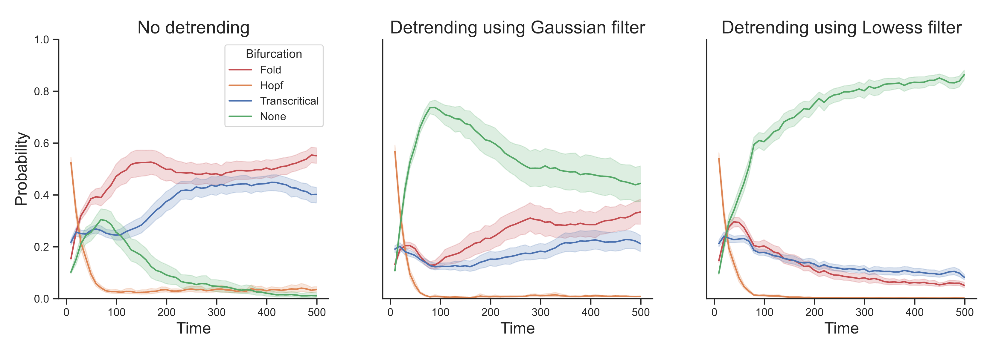
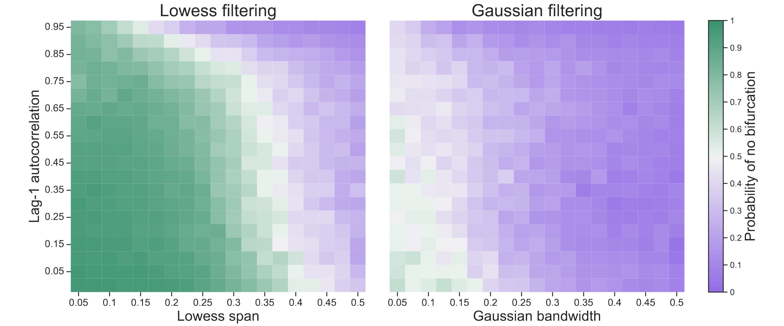

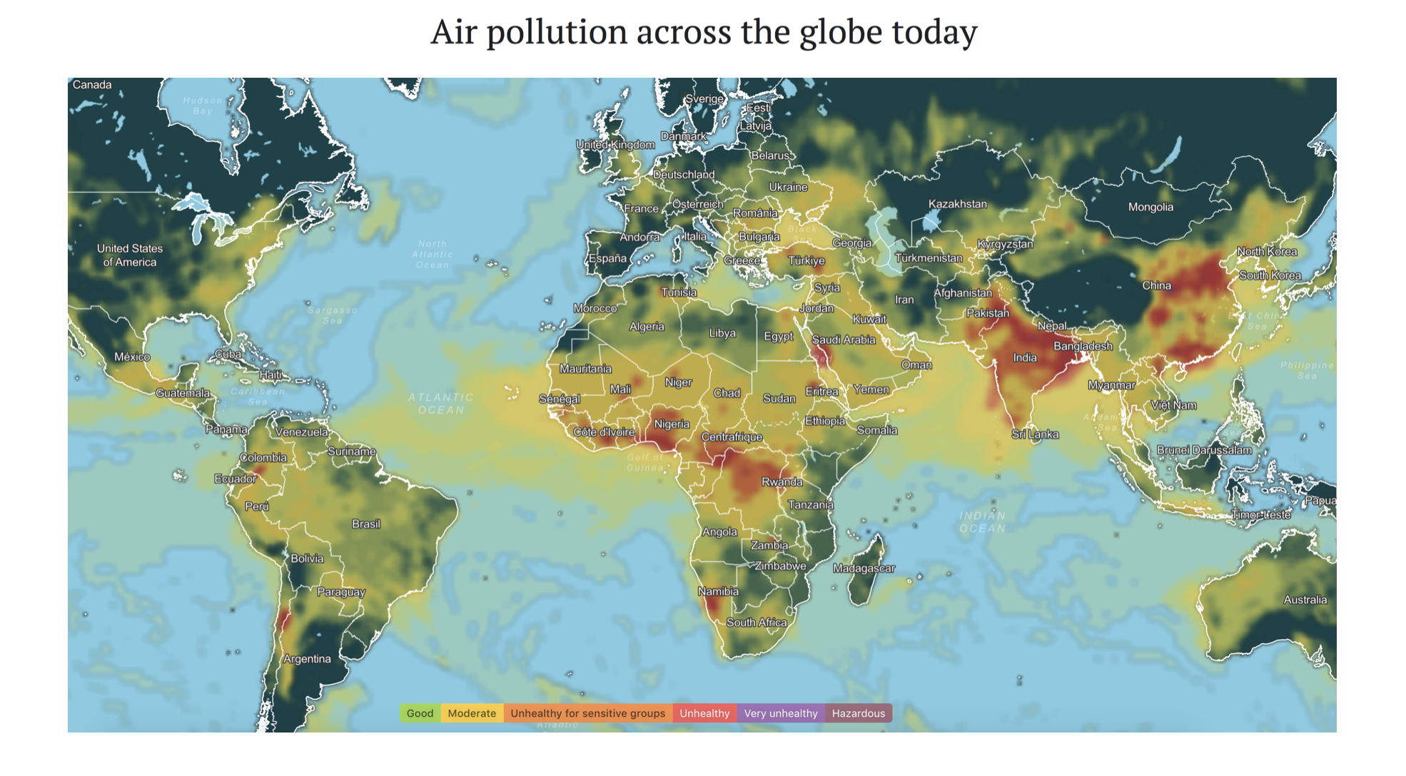
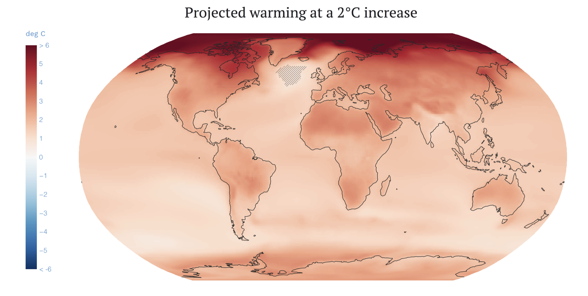
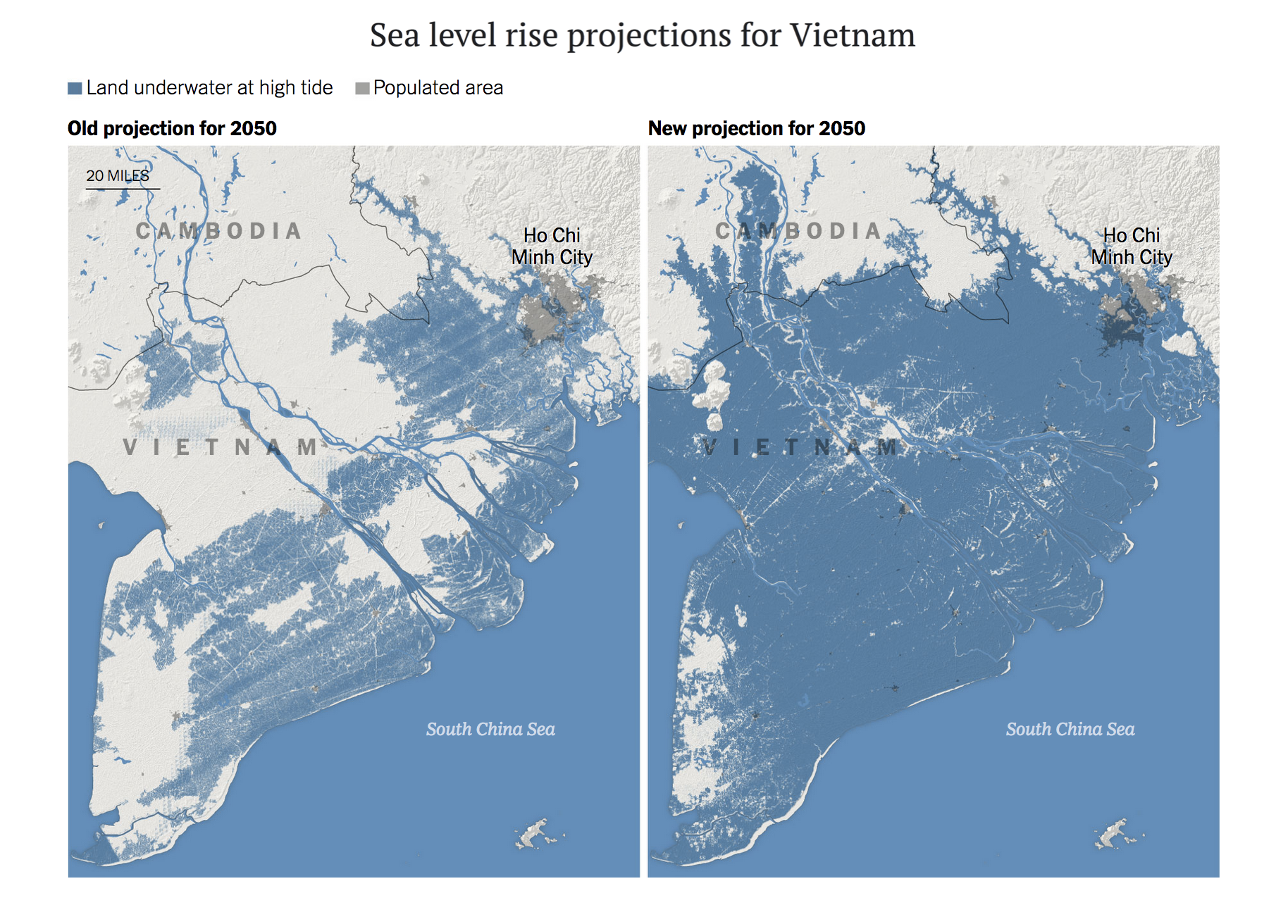
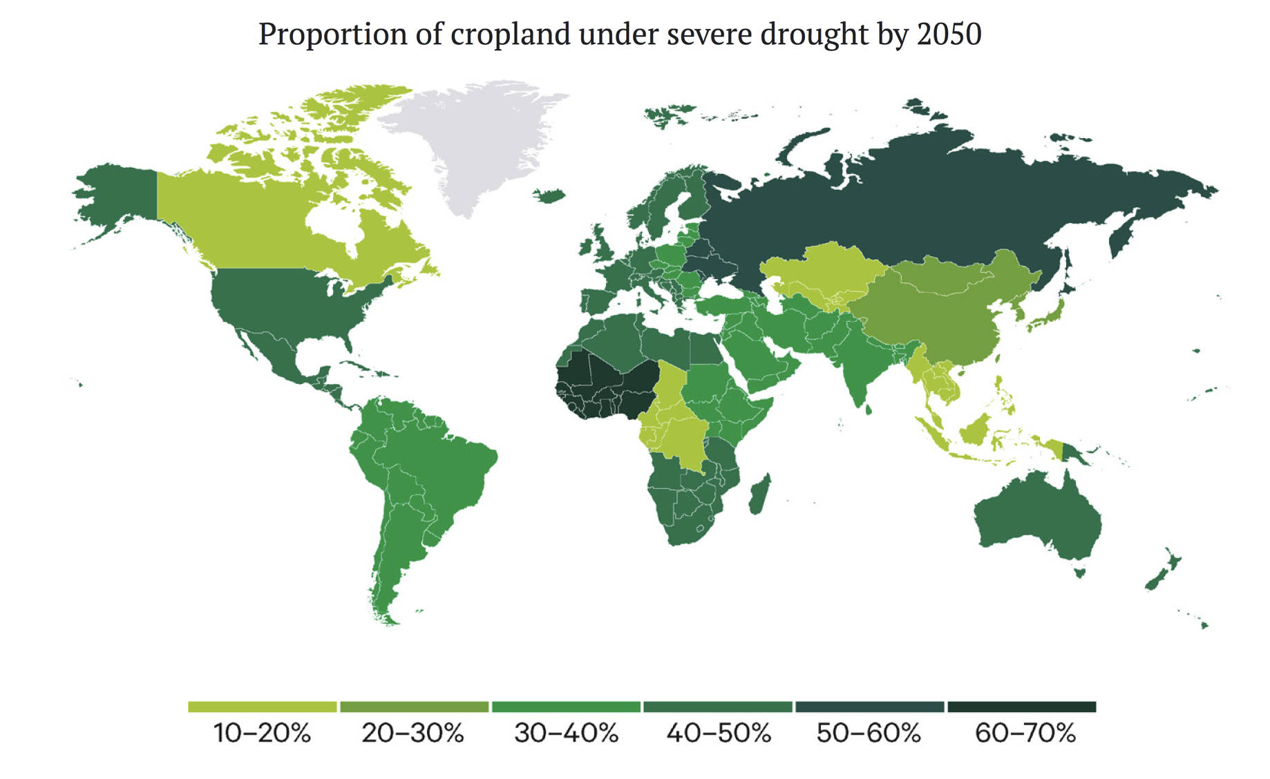
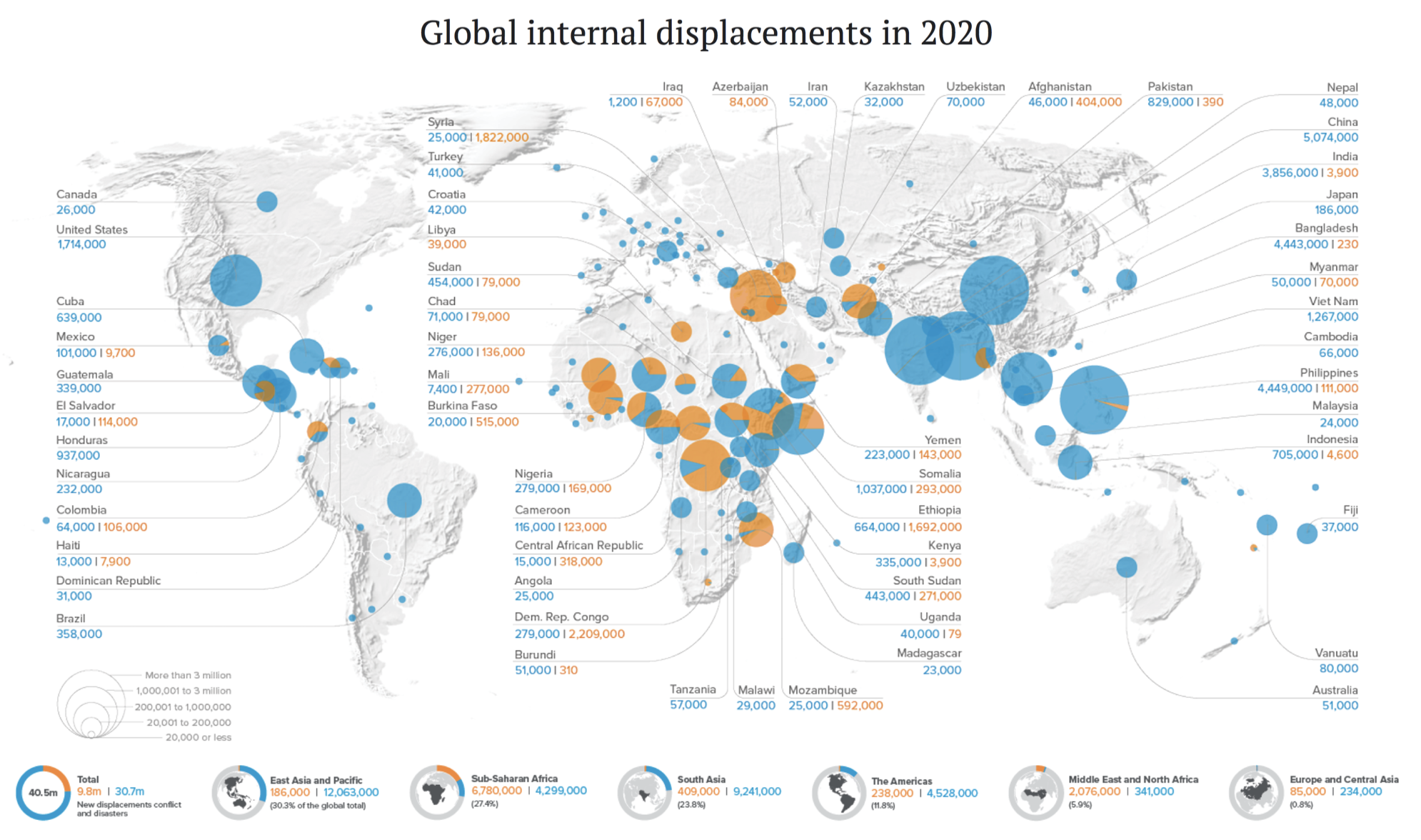
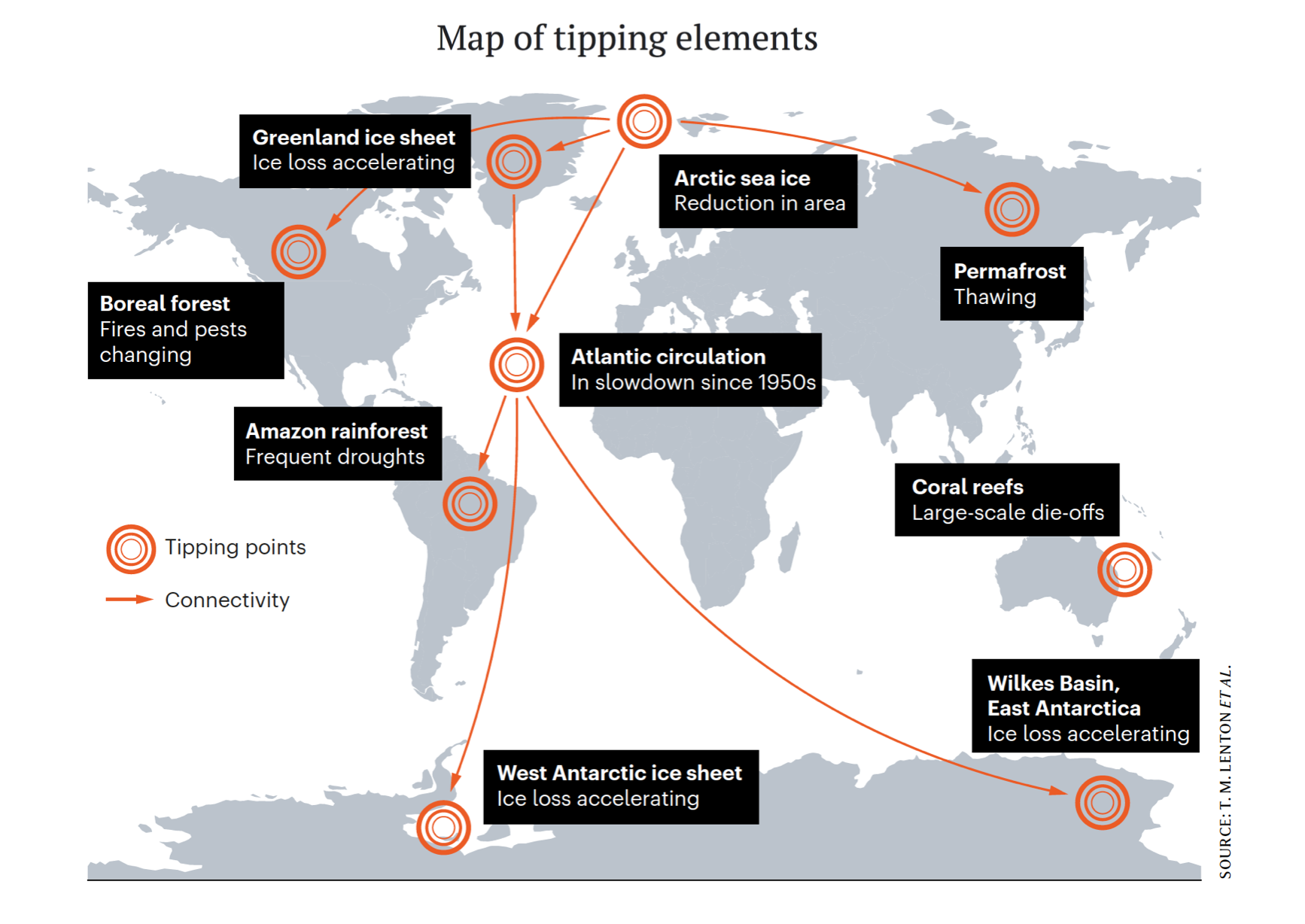
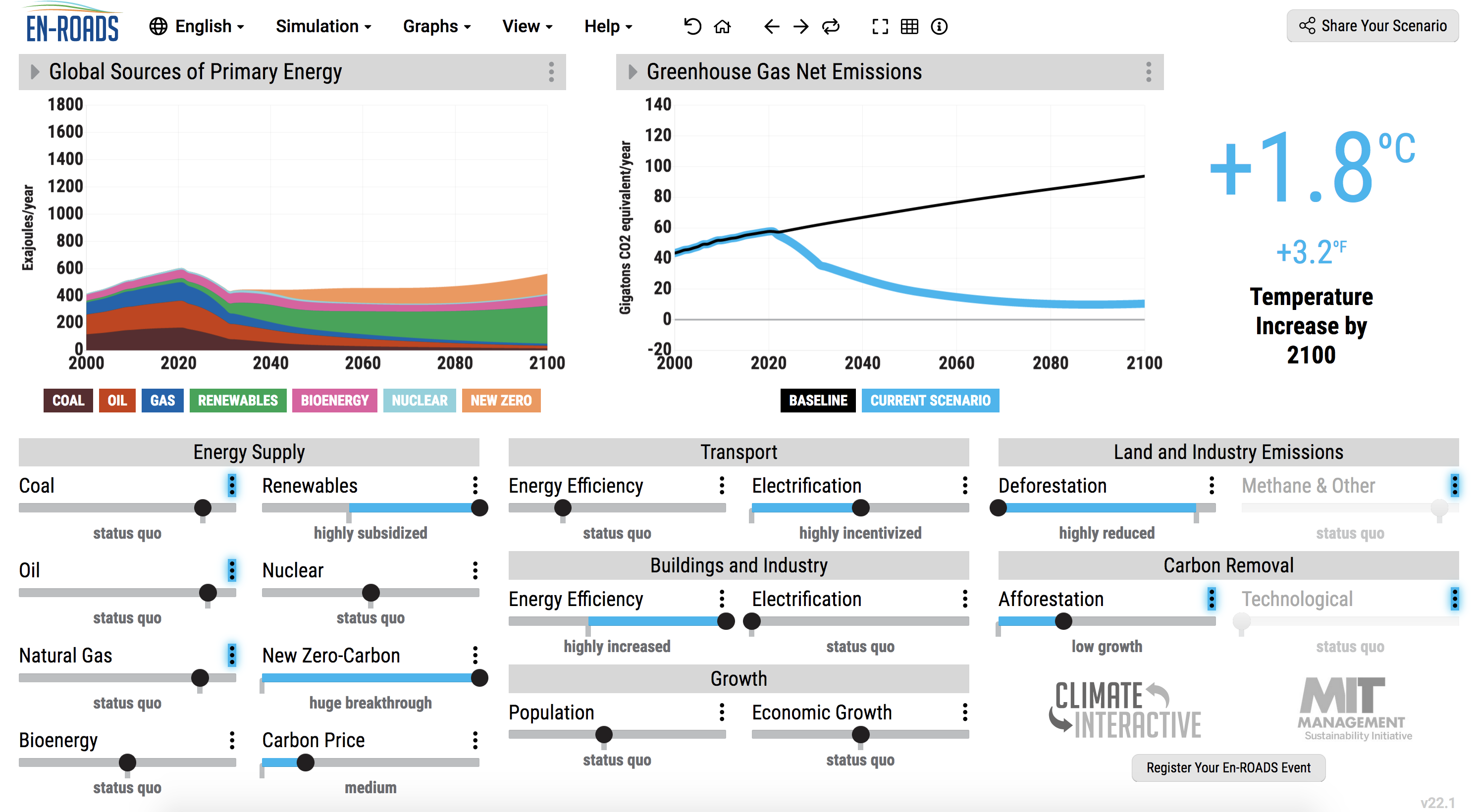
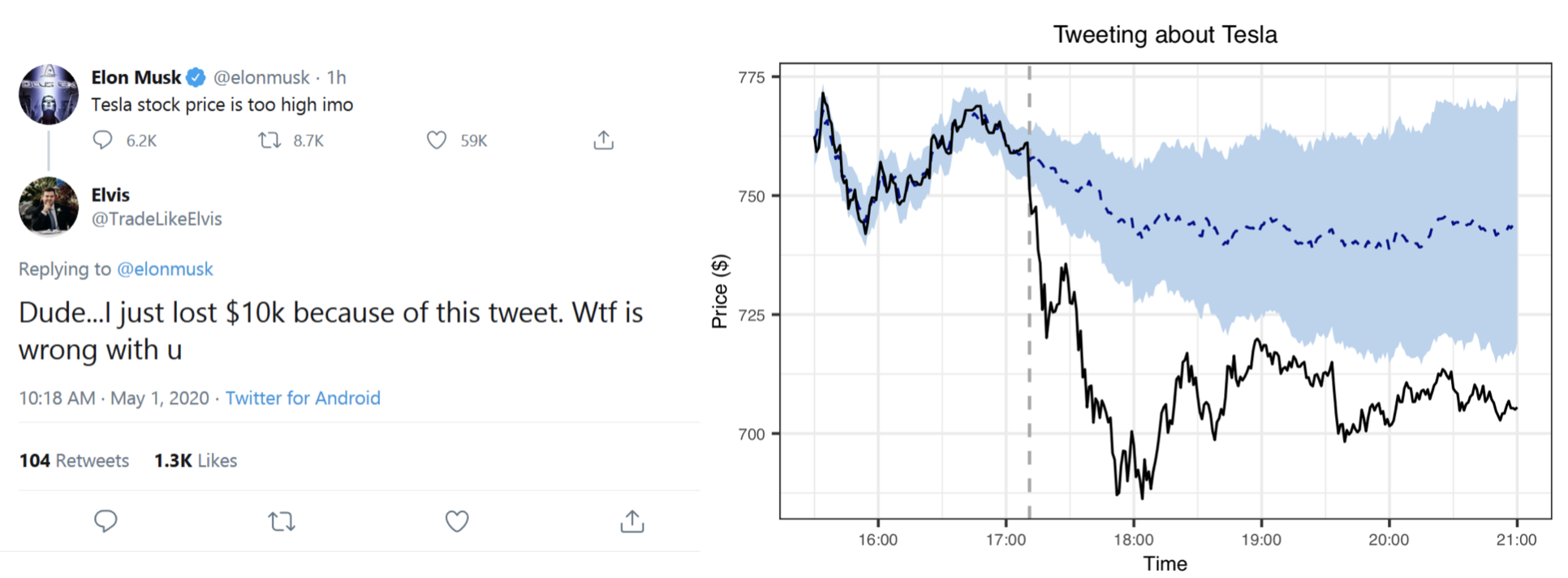


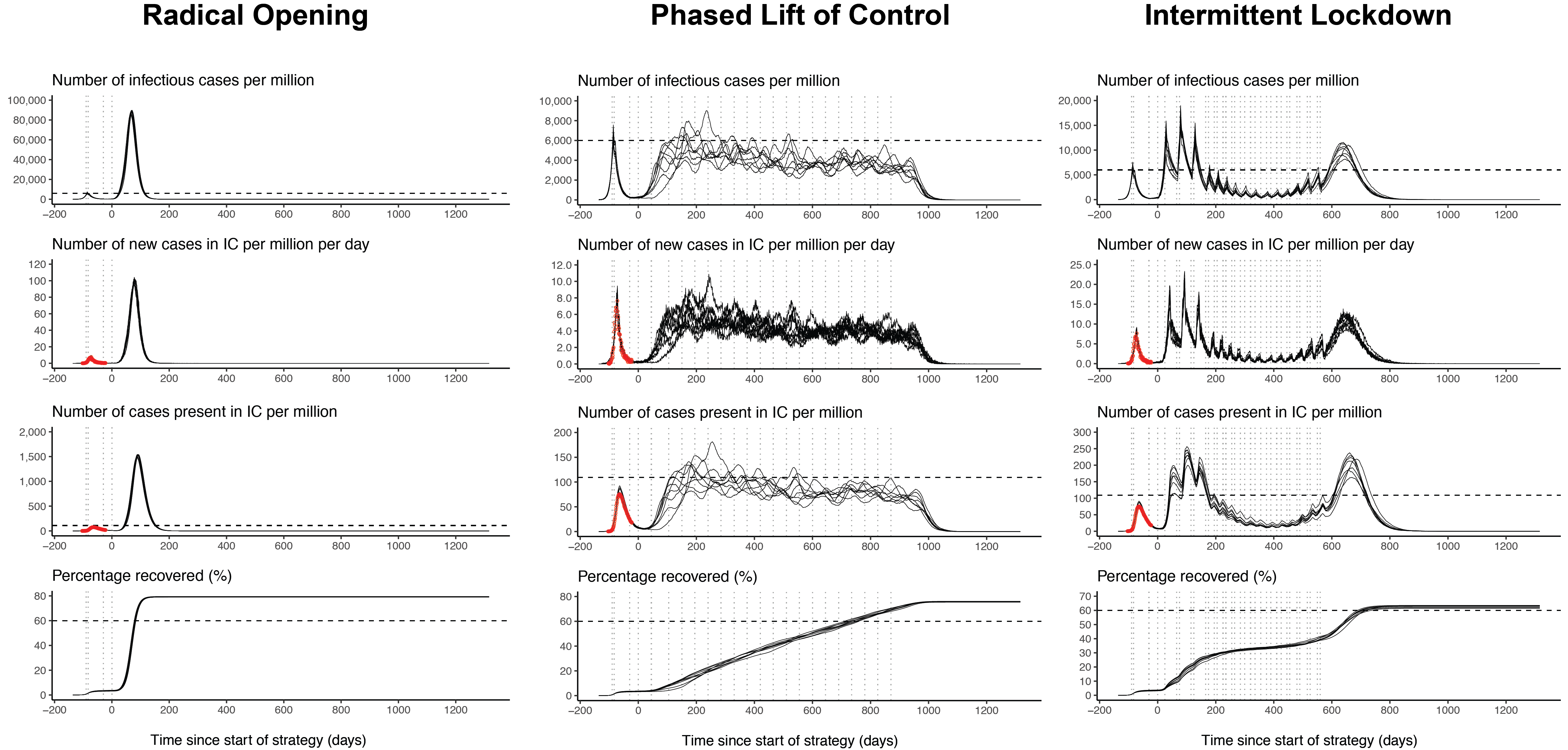
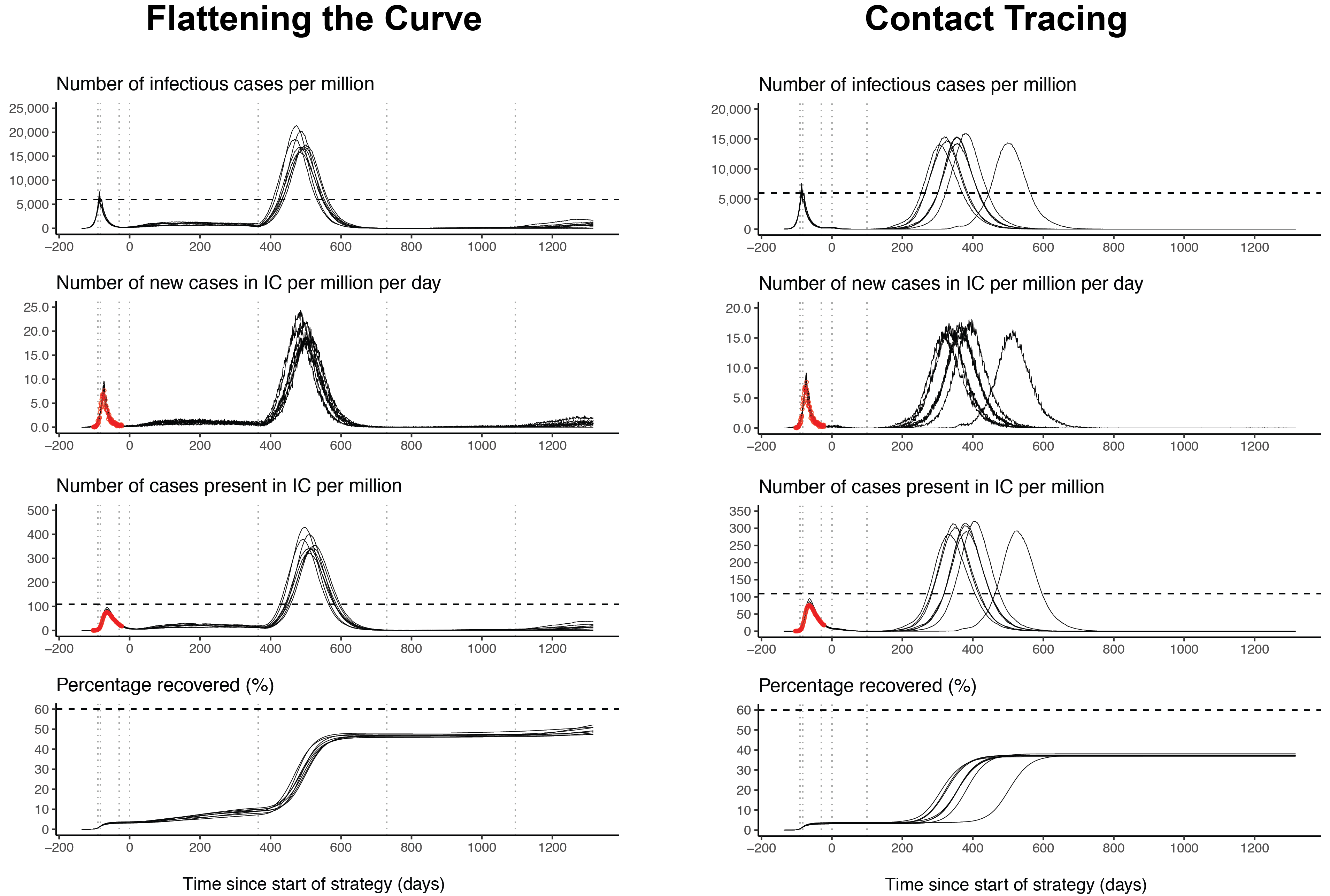


