Bayesian modeling using Stan: A case study

Practice makes better. And faster. But what exactly is the relation between practice and reaction time? In this blog post, we will focus on two contenders: the power law and exponential function. We will implement these models in Stan and extend them to account for learning plateaus and the fact that, with increased practice, not only the mean reaction time but also its variance decreases. We will contrast two perspectives on predictive model comparison: a (prior) predictive perspective based on marginal likelihoods, and a (posterior) predictive perspective based on leave-one-out cross-validation. So let’s get started!¹

Two models

We can model the relation between reaction time (in seconds) and the number of practice trials as a power law function. Let $f: \mathbb{N} \rightarrow \mathbb{R}^+$ be a function that maps the number of trials to reaction times. We write

where $\alpha$ is a lower bound (one cannot respond faster than that due to processing and motor control limits); $\beta$ is the learning gain from practice with respect to the first trial ($N = 1$); $N$ indexes the particular trial; and $r$ is the learning rate. Similarly, we can write

where the parameters have the same interpretation, except that $\beta$ is the learning gain from practice compared to no practice ($N = 0$).²

What is the main difference between those two functions? The exponential model assumes a constant learning rate, while the power model assumes diminishing returns. To see this, let $\alpha = 0$, and ignore for the moment that $N$ is discrete. Taking the derivative for the power law model results in

which shows that the local learning rate — the change in reaction time as a function of $N$ — is $-r/N$; it depends on how many trials have been completed previously. The more one has practiced, the smaller the local learning rate $-r / N$. The exponential function, in contrast, shows no such dependency on practice:

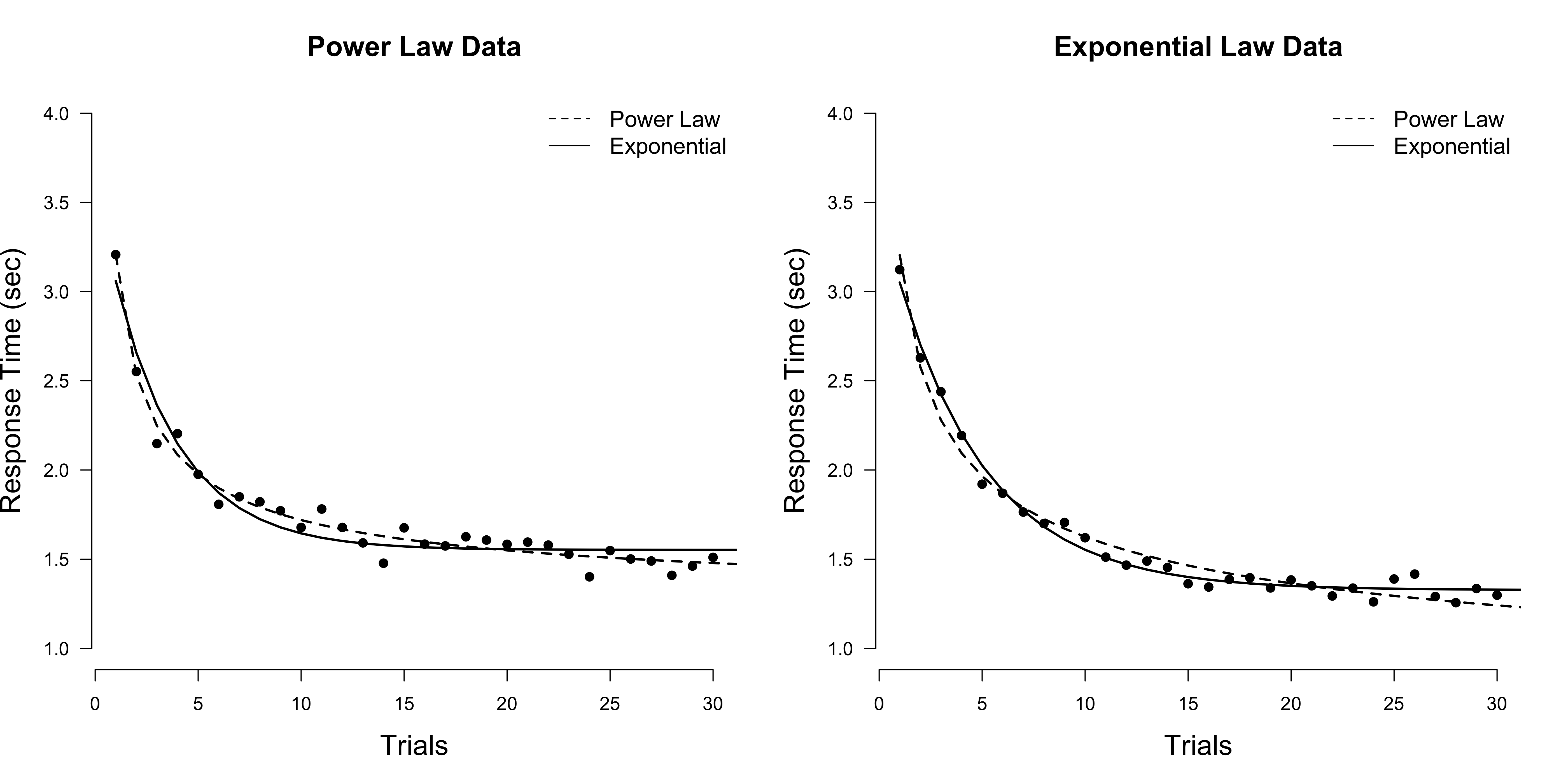
The figure above visualizes two data sets, generated from either a power law (left) or an exponential model (right), as well as the maximum likelihood fit of both models to these data. It is rather difficult to tell which model performs best just by eyeballing the fit. We thus need to engage in a more formal way of comparing models.

Two perspectives on prediction

Let’s agree that the best way to compare models is to look at predictive accuracy. Predictive accuracy with respect to what? The figure below illustrates two different answers one might give. The grey shaded surface represents unobserved data; the white island inside is the observed data; the model is denoted by $\mathcal{M}$.

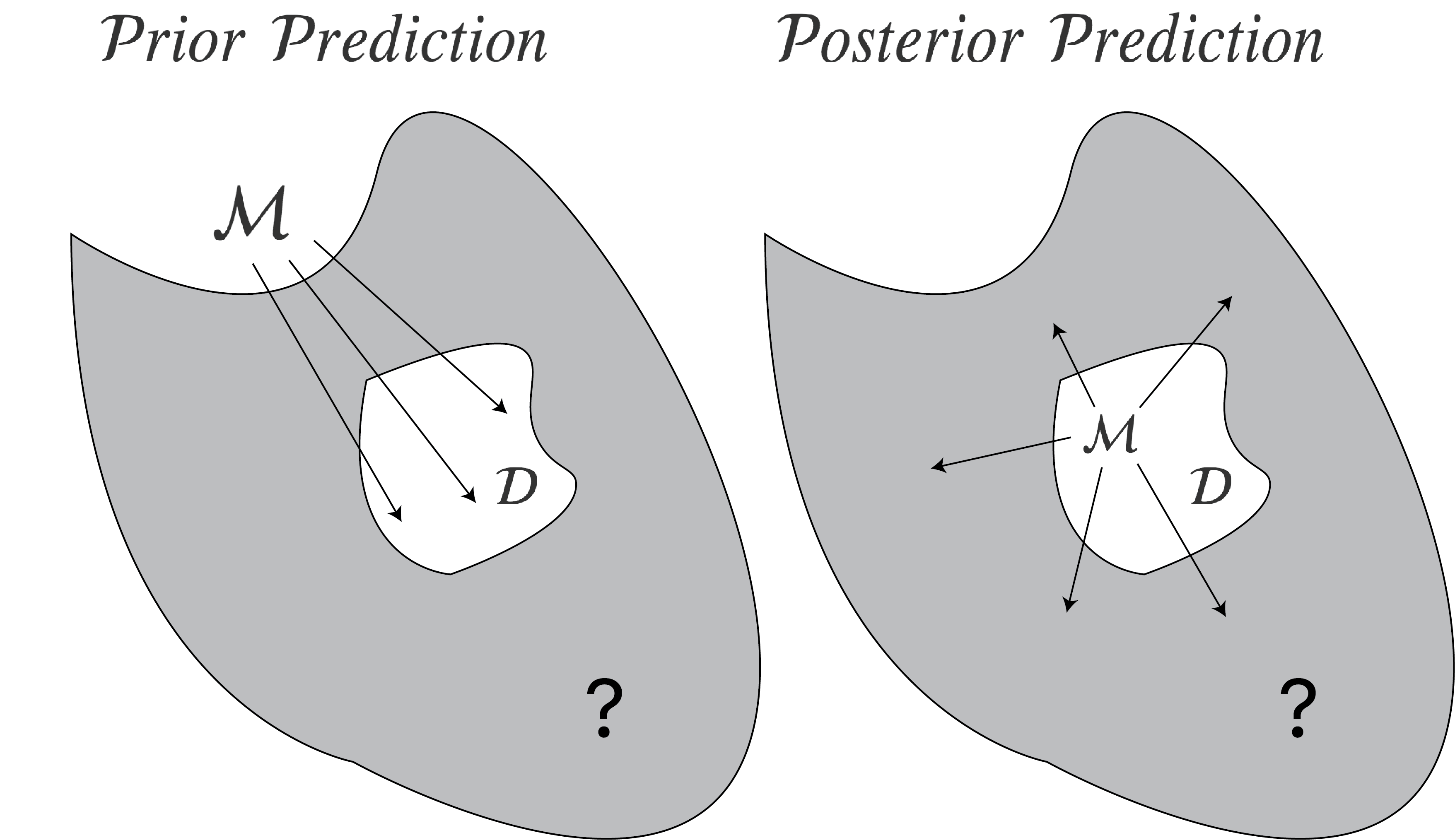
On the left, the model makes predictions before seeing any data by means of its prior predictive distribution. The predictive accuracy is then evaluated on the actually observed data. In contrast, on the right, the model makes predictions after seeing the data by means of its posterior predictive distribution. In principle, its predictive accuracy is evaluated on data one does not observe (visualized as the grey area). One can estimate this expected out-of-sample predictive accuracy by cross-validation procedures which partition the observed data into a training and test set. The model only sees the training set, and makes predictions for the unseen test set.

One key practical distinction between these two perspectives is how predictions are generated. On the left, predictions are generated from the prior. On the right, the prior first gets updated to the posterior using the observed data, and it is through the posterior that predictions are made. In the next two sections, we make this difference more precise.³

Prior prediction: Marginal likelihoods

From this perspective, we weight the model’s prediction of the observed data given a particular parameter setting by the prior. This is accomplished by integrating the likelihood with respect to the prior, which gives the so-called marginal likelihood of a model $\mathcal{M}$:

It is clear that the prior matters a great deal, but that is no surprise — it is part of the model. A bad prior means a bad model. The ratio of two such marginal likelihoods is known as the Bayes factor.

If one is willing to assign priors to models, one can compute posterior model probabilities, i.e.,

where $K$ is the number of models under consideration (see also a previous blogpost). Observe that the marginal likelihood features prominently: it is an updating factor from prior to posterior model probability. With this, one can also compute Bayesian model-averaged predictions:

where $\tilde{y}$ is unseen data, and where the prediction of each model gets weighted by its posterior probability. We denote a model weight, which in this case is its posterior probability, as $w_k$.

Posterior prediction: Leave-one-out cross-validation

Another perspective aims to estimate the expected out-of-sample prediction error, or expected log predictive density, i.e.,

where the expectation is taken with respect to unseen data $\tilde{y}$ (which is visualized as a grey surface with an $?$ inside in the figure above).

Clearly, as we do not have access to unseen data, we cannot evaluate this. However, one can approximate this quantity by computing the leave-one-out prediction error in our sample:

where $y_i$ is the $i^{\text{th}}$ data point, and $y_{-i}$ are all data points except $y_i$, where we have suppressed conditioning on $\mathcal{M}$ to not clutter notation (even more), and where

Observe that this requires integrating over the posterior distribution of $\theta$ given all but one data point; this is in contrast to the marginal likelihood perspective, which requires integration with respect to the prior distribution. From this perspective, one can similarly compute model weights $w_k$

where $\widehat{\text{elpd}}_{\text{loo}}^{\mathcal{M}_k}$ is the loo estimate for the expected log predictive density for model $\mathcal{M}_k$. For prediction, one averages across models using these Pseudo Bayesian model-averaging weights (Yao et al., 2018, p. 92).

However, Yao et al. (2018) and Vehtari et al. (2019) recommend against using these Pseudo BMA weights, as they do not take the uncertainty of the loo estimates into account. Instead, they suggest using Pseudo-BMA+ weights or stacking. For details, see Yao et al. (2018).

For an illuminating discussion about model selection based on marginal likelihoods or leave-one-out cross-validation, see Gronau & Wagenmakers (2019a), Vehtari et al. (2019), and Gronau & Wagenmakers (2019b).

Now that we have taken a look at these two perspectives on prediction, in the next section, we will implement the power law and the exponential model in Stan.

Implementation in Stan

As is common in psychology, people do not deterministically follow a power law or an exponential law. Instead, the law is probabilistic: given the same task, the person will respond faster or slower, never exactly as before. To allow for this, we assume that there is Gaussian noise around the function value. In particular, we assume that

Reaction times are known to not be normally distributed, however — we will address this later. We make the same assumption for the exponential model. The following code implements the power law model in Stan.

// In the data block, we specify everything that is relevant for
// specifying the data. Note that PRIOR_ONLY is a dummy variable used later.
 
data {
  int<lower=1> n;
  real y[n];
  int<lower=0, upper=1> PRIOR_ONLY;
}
 
 
// In the parameters block, we specify all parameters we need.
// Although Stan implicitly adds flat priors on the (positive) real line
// we will specify informative priors below.
 
parameters {
  real<lower=0> r;
  real<lower=0> alpha;
  real<lower=0> beta;
  real<lower=0> sigma_e;
}
 
// In the model block, we specify our informative priors and
// the likelihood of the model, unless we want to sample only from
// the prior (i.e., if PRIOR_ONLY == 1)
 
model {
  target += lognormal_lpdf(alpha | 0, .5);
  target += lognormal_lpdf(beta | 1, .5);
  target += gamma_lpdf(r | 1, 3);
  target += gamma_lpdf(sigma_e | 0.5, 5);
 
  if (PRIOR_ONLY == 0) {
    for (trial in 1:n) {
      target += normal_lpdf(y[trial] | alpha + beta * trial^(-r), sigma_e);
    }
  }
}
 
// In this block, we make posterior predictions (ypred) and compute
// the log likelihood of each data point (log_lik)
// which is needed for the computation of loo later
 
generated quantities {
  real ypred[n];
  real log_lik[n];
 
  for (trial in 1:n) {
    ypred[trial] = normal_rng(alpha + beta * trial^(-r), sigma_e);
    log_lik[trial] = normal_lpdf(y[trial] | alpha + beta * trial^(-r), sigma_e);
  }
 
}

From a marginal likelihood perspective, the prior is an integral part of the model; this means we have to think very carefully about it. There are several principles that can guide us (see also Lee & Vanpaemel, 2018), but one that is particularly helpful here is to look at the prior predictive distribution. Do draws from the prior predictive distribution look like what we had in mind? Below, I have visualized the mean, the standard deviation around the mean, and several draws from it for (a) flat priors on the positive real line, and (b) informed priors that I chose based on reading Evans et al. (2018). In the Stan code, you can specify flat priors by commenting out the priors we have specified in the model block.

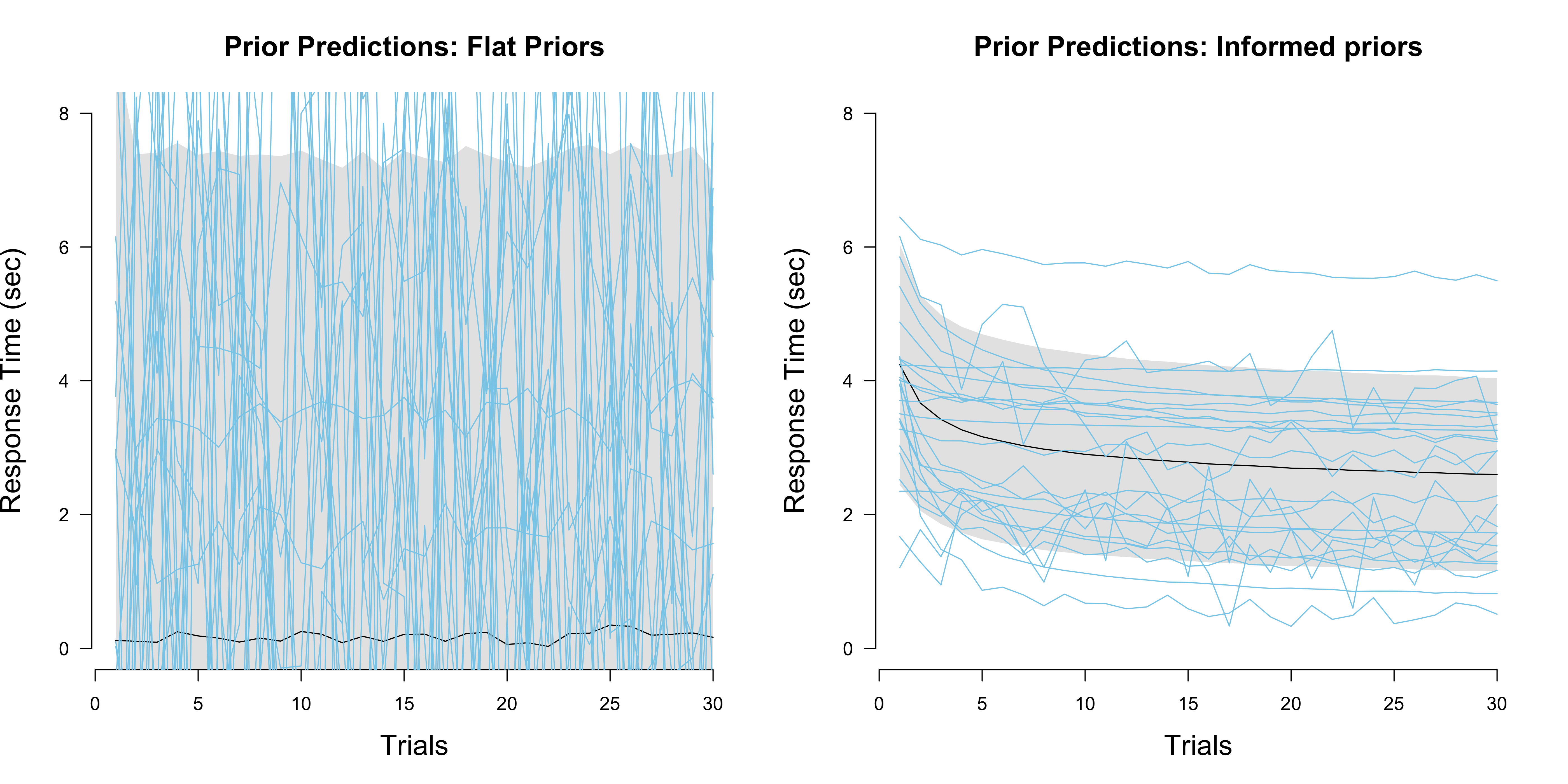
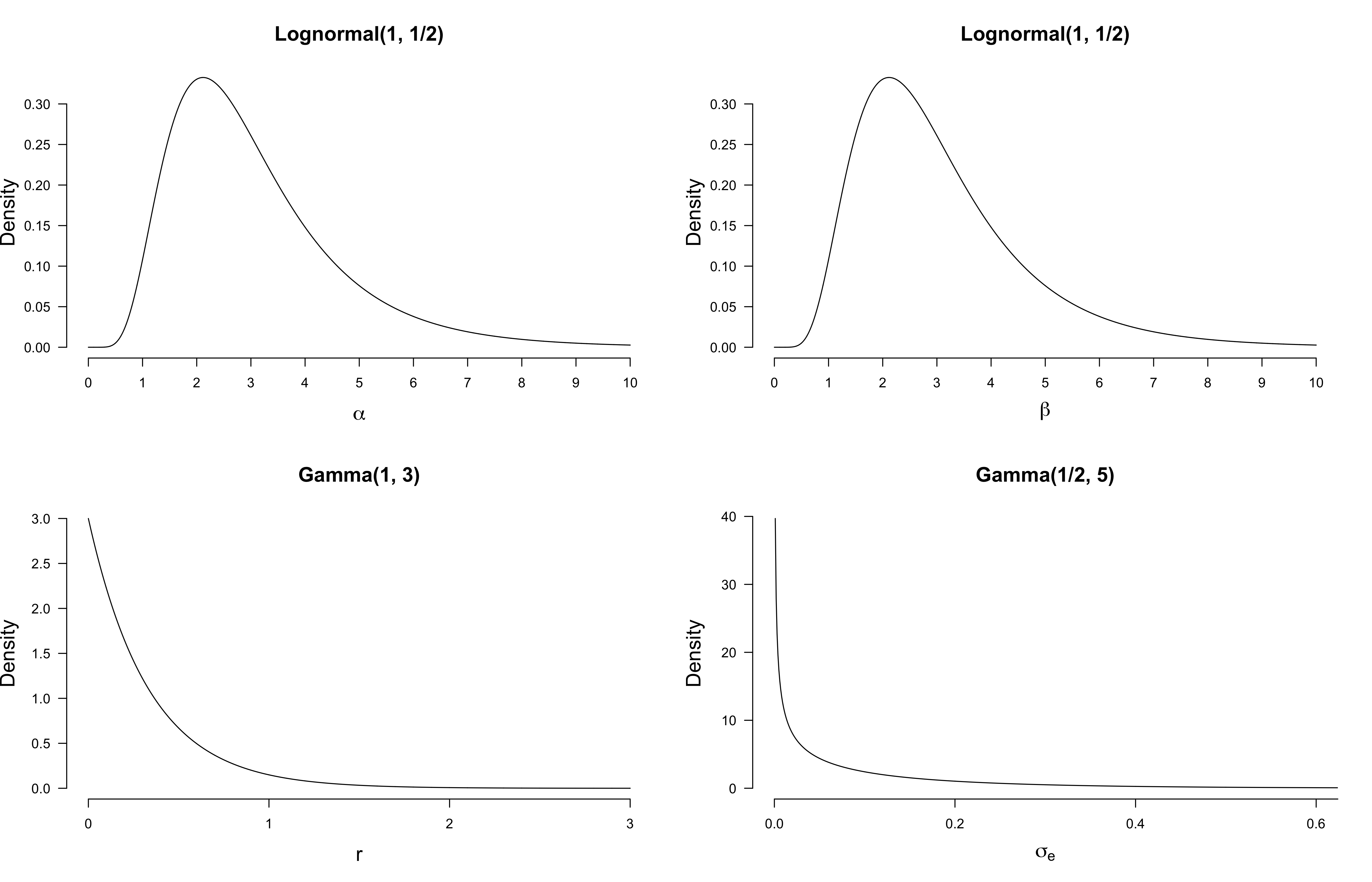
The Figure on the left shows that flat priors make terrible predictions. The mean of the prior predictive distribution is a constant function at zero, which is not at all what we had in mind when writing down the power law model. Even worse, flat priors allow for negative reaction time, something that is clearly impossible! In contrast, the Figure on the right seems reasonable. Below I have visualized the informed priors.

From a cross-validation perspective, priors do not matter that much; prediction is conditional on the observed data, and so the prior is transformed to a posterior before the model makes predictions. If the prior is not too misspecified, or if we have a sufficient amount of data so that the prior has only a weak influence on the posterior, a model’s posterior predictions will not markedly depend on it.

Practical model comparison

Let’s check whether we select the correct model for the power law and the exponential data, respectively. I have generated the data above using the following code, which will make sense later in the blog post.

sim_power <- function(N, alpha, beta, r, delta = 0, sdlog = 1) {
  delta + rlnorm(length(N), log(alpha + beta * N^(-r)), sdlog)
}
 
sim_exp <- function(N, alpha, beta, r, delta = 0, sdlog = 1) {
  delta + rlnorm(length(N), log(alpha + beta * exp(-r*N)), sdlog)
}
 
set.seed(1)
n <- 30
ns <- seq(n)
xp <- sim_power(ns, 1, 2, .7, .3, .05)
xe <- sim_exp(ns, 1, 2, .2, .3, .05)

We use the bridgesampling and the loo package to estimate Bayes factors and loo scores and stacking weights, respectively.

library('loo')
library('bridgesampling')
 
comp_power <- readRDS('stan-compiled/compiled-power-model.RDS')
comp_exp <- readRDS('stan-compiled/compiled-exponential-model.RDS')
 
# power model data
fit_pp <- sampling(
  comp_power,
  data = list('y' = xp, 'n' = n, 'PRIOR_ONLY' = 0),
  refresh = FALSE, chains = 4, iter = 8000, seed = 1
)
 
fit_ep <- sampling(
  comp_exp,
  data = list('y' = xp, 'n' = n, 'PRIOR_ONLY' = 0),
  refresh = FALSE, chains = 4, iter = 8000, seed = 1
)
 
# exponential data
fit_pe <- sampling(
  comp_power,
  data = list('y' = xe, 'n' = n, 'PRIOR_ONLY' = 0),
  refresh = FALSE, chains = 4, iter = 8000, seed = 1
)
 
fit_ee <- sampling(
  comp_exp,
  data = list('y' = xe, 'n' = n, 'PRIOR_ONLY' = 0),
  refresh = FALSE, chains = 4, iter = 8000, seed = 1
)

But before we do so, let’s visualize the posterior predictions of both models for each simulated data set, respectively.

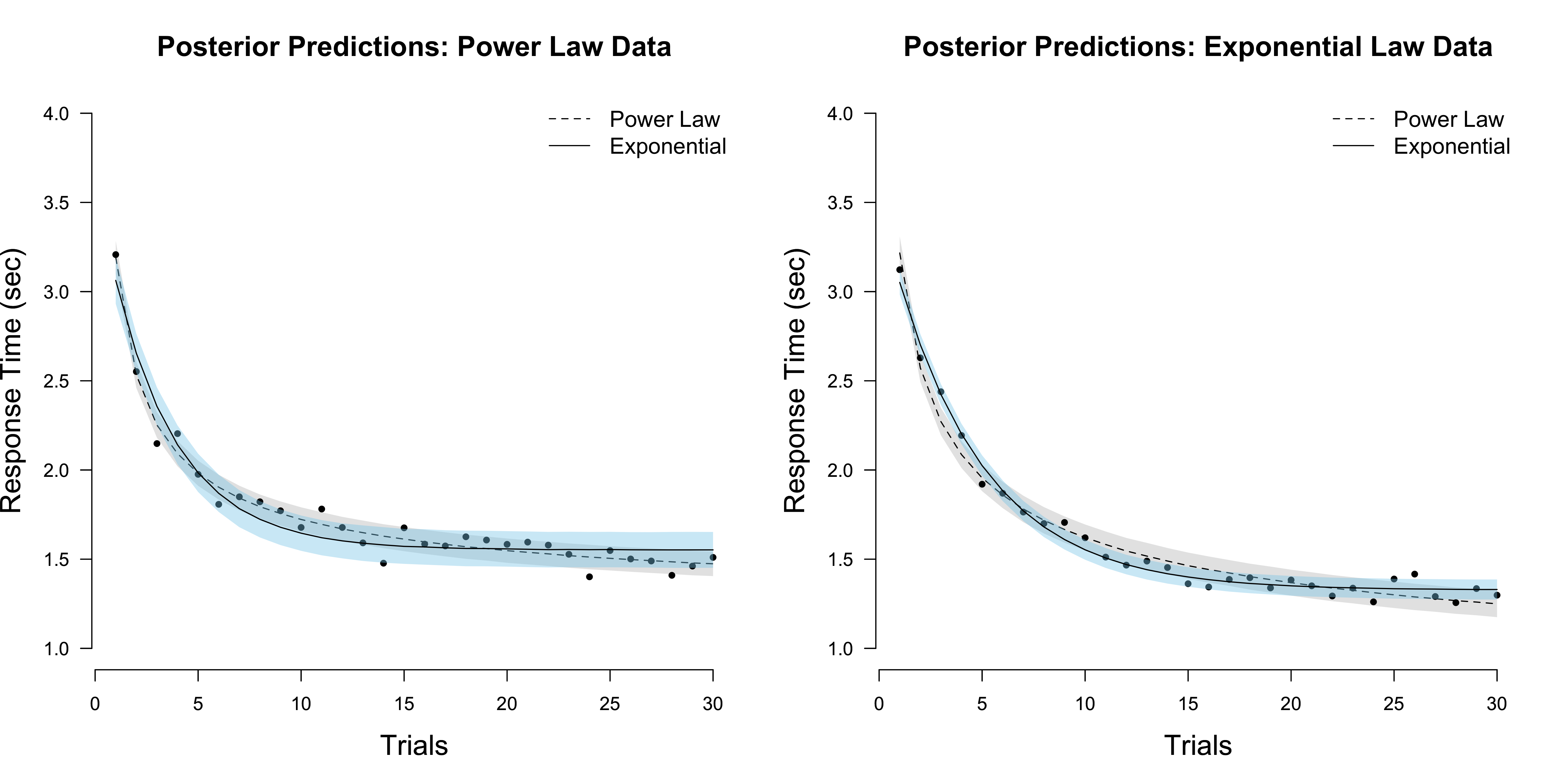
In the figure on the left, we see that the posterior predictions for the exponential model have a larger variance compared to the predictions of the power law model. Conversely, on the right it seems that the exponential model gives the better predictions.⁴

We first compare the two models on the power law data, using the Bayes factor and loo. With the former, we find overwhelming evidence in favour of the power law model.

bayes_factor(
  bridge_sampler(fit_pp, silent = TRUE),
  bridge_sampler(fit_ep, silent = TRUE)
)

## Estimated Bayes factor in favor of x1 over x2: 54950.14619

Note that this estimate can vary with different runs (since we were stingy in sampling from the posterior). The comparison using loo yields the following output:

loo_pp <- loo(fit_pp)

## Warning: Some Pareto k diagnostic values are too high. See help('pareto-k-diagnostic') for details.

loo_ep <- loo(fit_ep)

## Warning: Some Pareto k diagnostic values are too high. See help('pareto-k-diagnostic') for details.

loo_compare(loo_pp, loo_ep)

##        elpd_diff se_diff
## model1   0.0       0.0  
## model2 -14.2       5.4

Note that the best model is always on top, and the comparison is already on the difference score. Following a two standard error heuristic (but see here), since the difference in the elpd scores is more than twice its standard error, we would choose the power law model as the better model. But wait – what do these warnings mean? Let’s look at the output of the loo function for the exponential law (suppressing the warning):

loo_ep

## 
## Computed from 16000 by 30 log-likelihood matrix
## 
##          Estimate   SE
## elpd_loo     22.9  5.7
## p_loo         7.4  3.9
## looic       -45.8 11.5
## ------
## Monte Carlo SE of elpd_loo is NA.
## 
## Pareto k diagnostic values:
##                          Count Pct.    Min. n_eff
## (-Inf, 0.5]   (good)     28    93.3%   6801      
##  (0.5, 0.7]   (ok)        1     3.3%   369       
##    (0.7, 1]   (bad)       0     0.0%   <NA>      
##    (1, Inf)   (very bad)  1     3.3%   9         
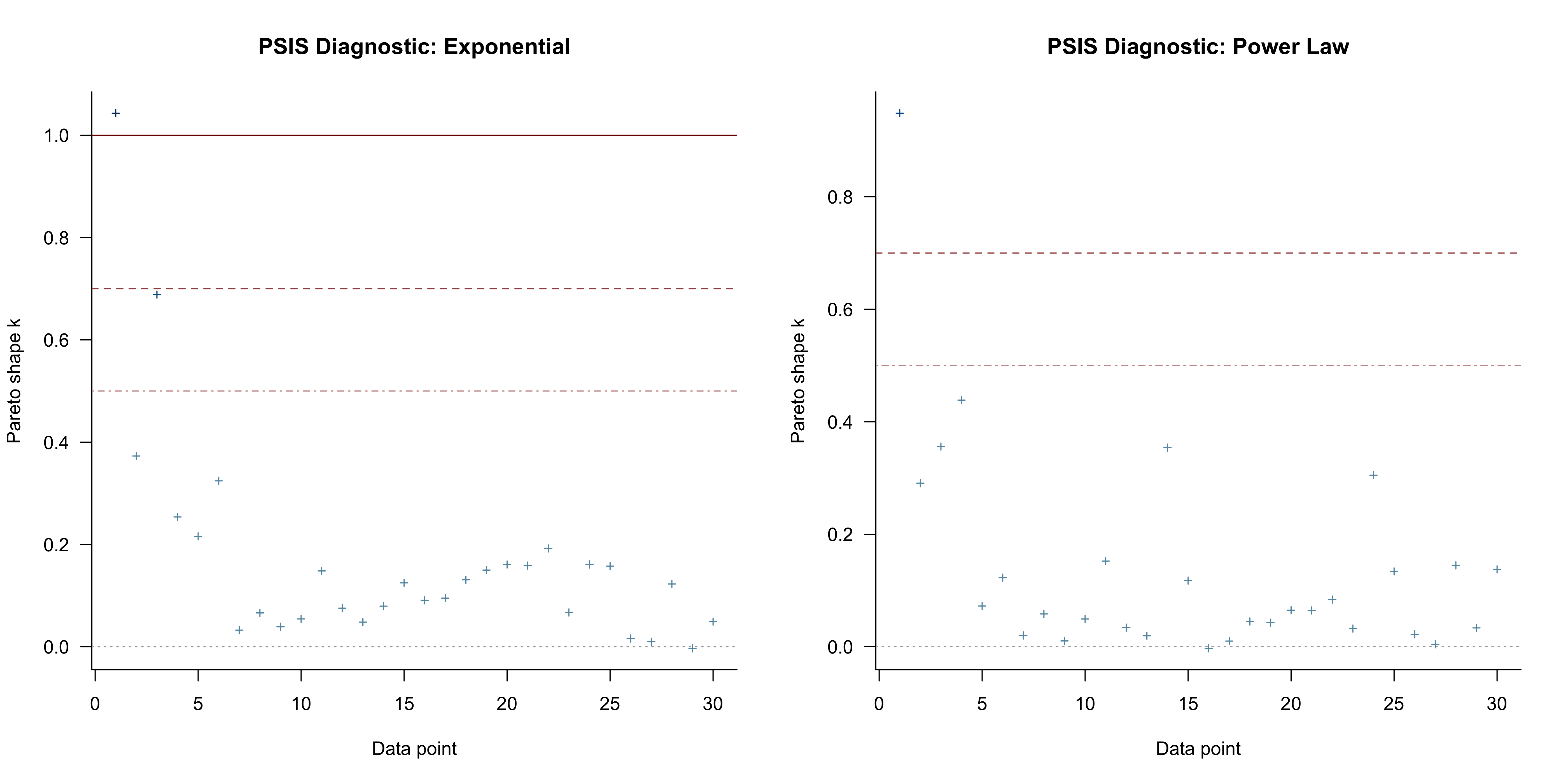
## See help('pareto-k-diagnostic') for details.

We find that there are is one very bad Pareto $k$ value. What does this mean? There are many details about loo that you can read up on in Vehtari et al. (2018). Put briefly, to efficiently compute the loo score of a model, Vehtari et al. (2018) use importance sampling to compute the predictive density, which requires finding importance weights to better approximate this density. These importance weights are known to be unstable, and the authors introduce a particular stabilizing transformation which they call “Pareto smoothed importance sampling” (PSIS). The parameter $k$ is the shape parameter of this (generalized) Pareto distribution. If it is high, such as $k > 0.7$ as we find for one data point here, then this implies unstable estimates — we should probably not trust the loo estimate for this model.⁵ Similarly pathological behaviour can be diagnosed by p_loo, which gives an estimate of the effective number of parameters. In this case, this is about double the number of actual parameters ($\alpha, \beta, r, \sigma_e^2$).

The two figures below visualize the $k$ values for each data point. We see that loo has troubles predicting the first data point for both the exponential and power law model.

We can also compute the stacking weights; but again, one should probably not trust these estimates:

stacking_weights <- function(fit1, fit2) {
  log_lik_list <- list(
    '1' = extract_log_lik(fit1),
    '2' = extract_log_lik(fit2)
  )
  
  r_eff_list <- list(
    '1' = relative_eff(extract_log_lik(fit1, merge_chains = FALSE)),
    '2' = relative_eff(extract_log_lik(fit2, merge_chains = FALSE))
  )
  
  loo_model_weights(log_lik_list, method = 'stacking', r_eff_list = r_eff_list)
}
 
stacking_weights(fit_pp, fit_ep)

## Method: stacking
## ------
##   weight
## 1 0.995 
## 2 0.005

We could compute a “Stacked Pseudo Bayes factor” by taking the ratio of these two weights to see how much more weight one model is given compared to the other.⁶ This yields a factor of about 120 in favour of the power law model.

We can make the same comparisons using the exponential data. The Bayes factor again yields overwhelming support for the model that is closer to the true model, i.e., in this case the exponential model.⁷ But note that the evidence is an order of magnitude smaller than in the above comparison.

bayes_factor(
  bridge_sampler(fit_ee, silent = TRUE),
  bridge_sampler(fit_pe, silent = TRUE)
)

## Estimated Bayes factor in favor of x1 over x2: 1024.51382

This marked decrease in evidence is also tracked by loo, which now tells us that we cannot reliably distinguish between the two models⁸:

loo_compare(loo(fit_ee), loo(fit_pe))

## Warning: Some Pareto k diagnostic values are too high. See help('pareto-k-diagnostic') for details.

## Warning: Some Pareto k diagnostic values are too high. See help('pareto-k-diagnostic') for details.

##        elpd_diff se_diff
## model1  0.0       0.0   
## model2 -8.3       5.6

Note that while we still get warnings, this time we only have one data point with $k \in [0.7, 1]$, which is bad, but not very bad. The stacking weights show that there is not a clear winner, with a factor of only about 6 in favour of the exponential model:

stacking_weights(fit_ee, fit_pe)

## Method: stacking
## ------
##   weight
## 1 0.847 
## 2 0.153

Now that we have seen how one might compare these models in practice, in the next two sections, we will see how we can extend the model to be more realistic. To that end, I will focus only on the exponential model. In fact, the exponential model is what many researchers now prefer as the “law of practice”. In a very influential article, Newell & Rosenbloom (1981) found that a power law fit best for data from a wide variety of tasks. While they relied on averaged data, Heathcote et al. (2000) looked at participant-specific data. They found that the decrease in reaction time follows an exponential function, implying that previous results were biased due to averaging; in fact, one can show that the (arithmetic) averaging of many exponential (i.e., non-linear) functions can lead to a group-level power law when individual differences exist (Myung, Kim, & Pitt, 2000).

Extension I: Modeling plateaus

The above two models assume that participants get it from the first trial onwards, and become better immediately. However, real data often exhibits a plateau. We simulate such data using the following lines of code.

set.seed(1)
dat <- c(
  rlnorm(15, 1.25, .1),
  sim_exp(seq(16, 50), 2, 5, .1, 0, .1)
)

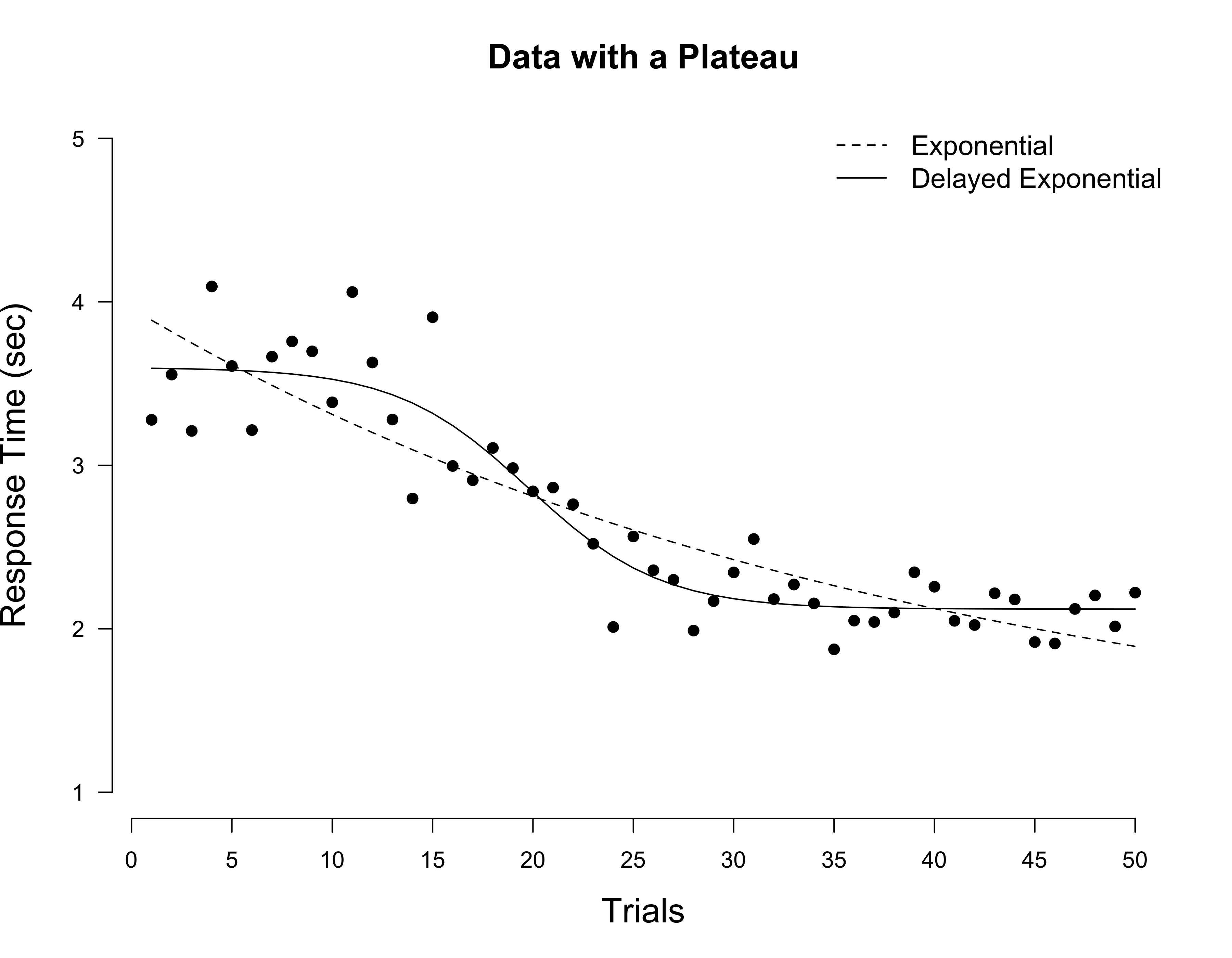
How can we model this? Evans et al. (2018) suggest introducing a single parameter, $\tau$, and adjusting the model as follows:

Observe that for $\tau = 0$, we recover the original exponential model. For $\tau \rightarrow \infty$, the function becomes a constant function $\alpha + \beta$. Thus, large values for $\tau$ (and large values for $r$, so as to model the steep drop in reaction time) allow us to model the initial plateau we find in real data.

We can adjust the model in Stan easily:

data {
  int<lower=1> n;
  real y[n];
  int<lower=0, upper=1> PRIOR_ONLY;
}
 
parameters {
  real<lower=0> r;
  real<lower=0> alpha;
  real<lower=0> beta;
  real<lower=0> sigma_e;
  real<lower=0> tau;
}
 
model {
  real mu;
  // Renormalize Cauchy prior due to truncation to get correct marginal likelihood
  target += cauchy_lpdf(tau | 0, 1) - cauchy_lccdf(0 | 0, 1);
  target += lognormal_lpdf(alpha | 0, .5);
  target += lognormal_lpdf(beta | 1, .5);
  target += gamma_lpdf(r | 1, 3);
  target += gamma_lpdf(sigma_e | 0.5, 5);
 
  if (PRIOR_ONLY == 0) {
    for (trial in 1:n) {
      mu = alpha + beta * (tau + 1) / (tau + exp(r * trial));
      target += normal_lpdf(y[trial] | mu, sigma_e);
    }
  }
}
 
generated quantities {
  real mu;
  real ypred[n];
  real log_lik[n];
 
  for (trial in 1:n) {
    mu = alpha + beta * (tau + 1) / (tau + exp(r * trial));
    ypred[trial] = normal_rng(mu, sigma_e);
    log_lik[trial] = normal_lpdf(y[trial] | mu, sigma_e);
  }
 
}

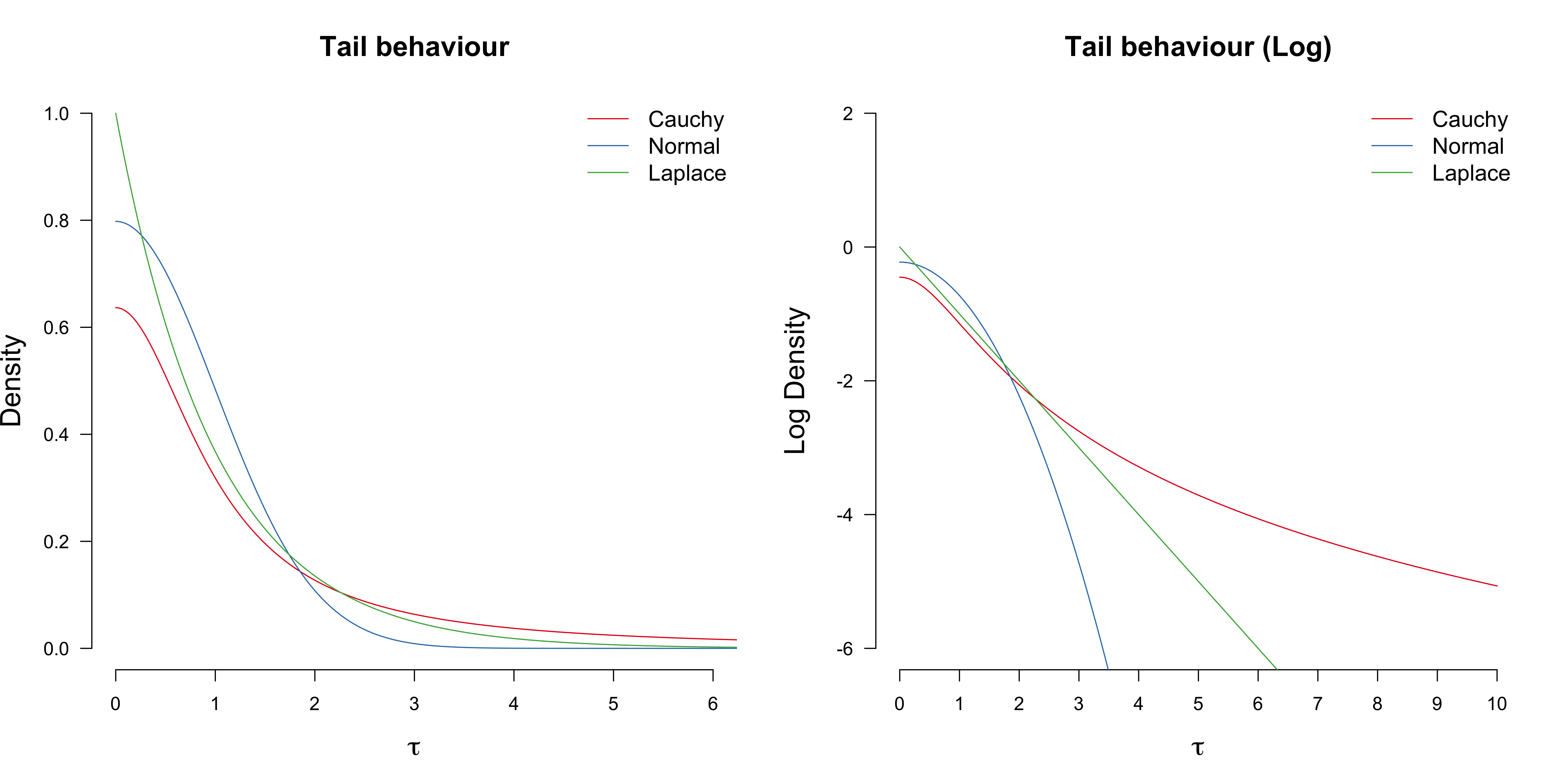
We have put a half-Cauchy prior on $\tau$. This is because the Cauchy distribution has very fat tails, compared to for example the Normal or the Laplace distribution; see Figure below. This is desired, because we need large $\tau$ values to accommodate plateaus.

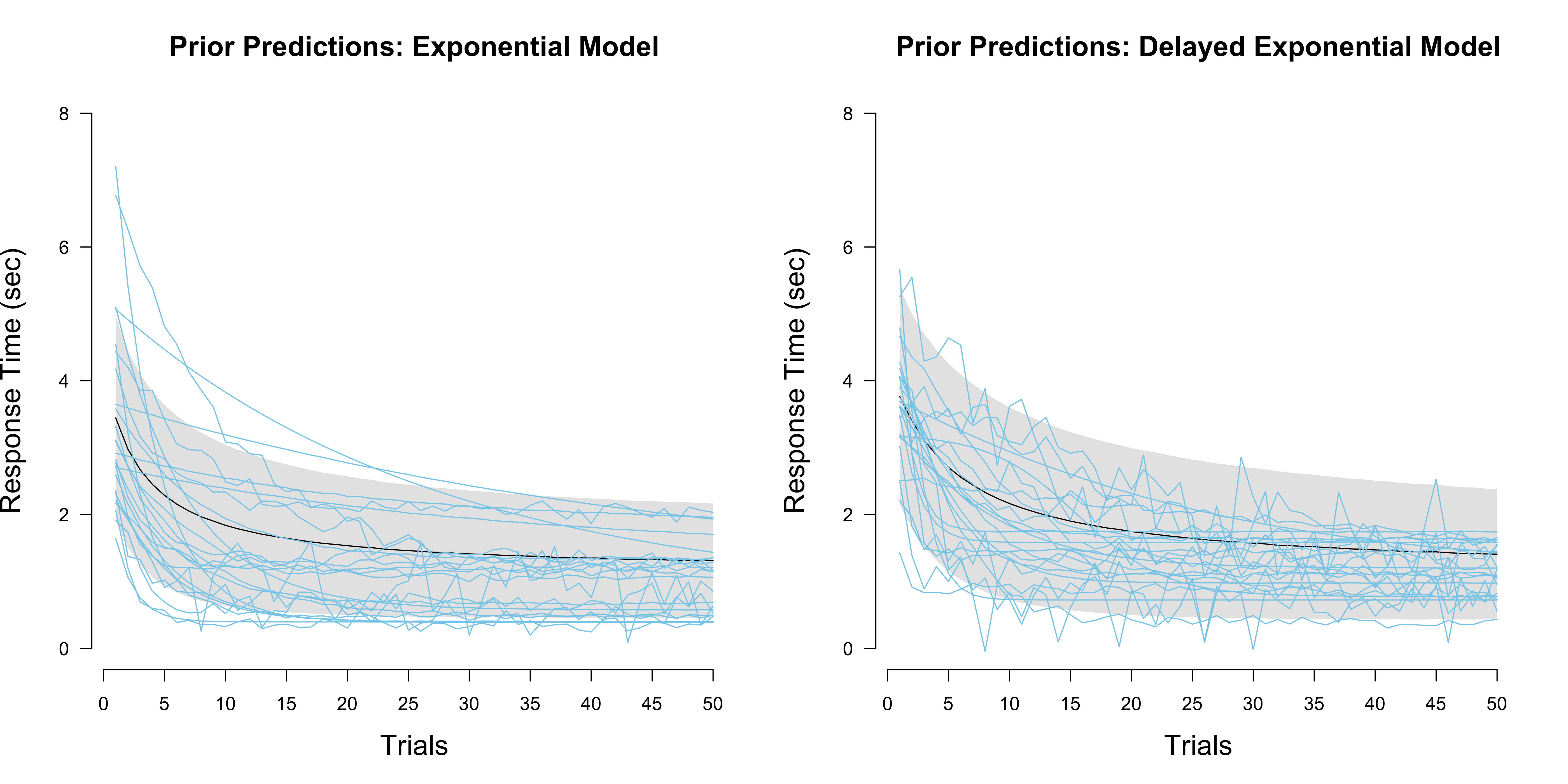
The figure below compares the prior predictive distributions of the exponential to the delayed exponential model. As we can see, the additional $\tau$ parameter creates larger uncertainty in the predictions, with the some individual draws looking completely different from each other. Drawing samples from a Cauchy, whose mean and variance are undefined, is tricky.

However, if we compare the two models to each other on the plateau data set, we see that the extended model predicts the data better:

fit_ee <- sampling(
  comp_exp,
  data = list('y' = dat, 'n' = 50, 'PRIOR_ONLY' = 0),
  refresh = FALSE, chains = 4, iter = 8000, seed = 1
)
 
fit_ee_plateau <- sampling(
  comp_exp_delayed,
  data = list('y' = dat, 'n' = 50, 'PRIOR_ONLY' = 0),
  refresh = FALSE, chains = 4, iter = 8000, seed = 1
)
 
bayes_factor(
  bridge_sampler(fit_ee_plateau, silent = TRUE, method = 'warp3'),
  bridge_sampler(fit_ee, silent = TRUE, method = 'warp3')
)

## Estimated Bayes factor in favor of x1 over x2: 304.35681

This is a large Bayes factor. However, loo seems to favour the delayed exponential model much more, by about three standard errors:

loo_compare(loo(fit_ee_plateau), loo(fit_ee))

##        elpd_diff se_diff
## model1   0.0       0.0  
## model2 -10.4       3.3

This is also reflected in an extreme difference in stacking weights, which completely discounts the standard exponential model:

stacking_weights(fit_ee_plateau, fit_ee)

## Method: stacking
## ------
##   weight
## 1 1.000 
## 2 0.000

Earlier, when comparing the exponential and power model on data generated from an exponential model, we found a Bayes factor in favour of the exponential model of about 1000, while the difference in loo was only about 1.5 standard errors. Here, we now find a Bayes factor in favour of the delayed exponential model of only about 300, while loo finds a difference of about three standard errors. This contrast becomes is illuminated by visualizing the posterior predictive distribution, see below.

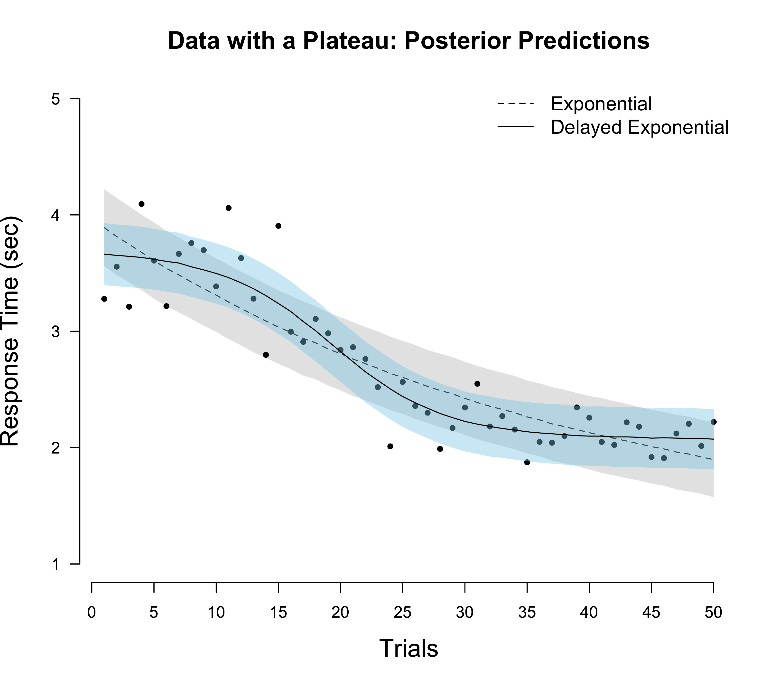
We see that the delayed exponential model seems to “fit” the data much better.⁹ Since loo basically uses this posterior predictive distribution (except that it removes one data point) to predict individual data points, it now seems clearer why it should favour the delayed exponential model so much more strongly. In contrast, the prior predictive distributions of the exponential and the delayed exponential (visualized above) are rather similar. Since the Bayes factor evaluated the probability of the data given these prior predictive distributions, the evidence in favour of the delayed exponential model is only modest.

Extension II: Modeling reaction times

The Lognormal distribution

Reaction times are well known to be non-normally distributed. One popular distribution for them is the Lognormal distribution. Let $X \sim \mathcal{N}(\mu, \sigma^2)$. Then $Z = e^X$ is lognormally distributed. To arrive at its density function, we do a change of variables. Observe that

where $F_x$ is the cumulative distribution function of $X$. Differentiating with respect to $z$ yields the probability density function for $Z$:

which spelled out is

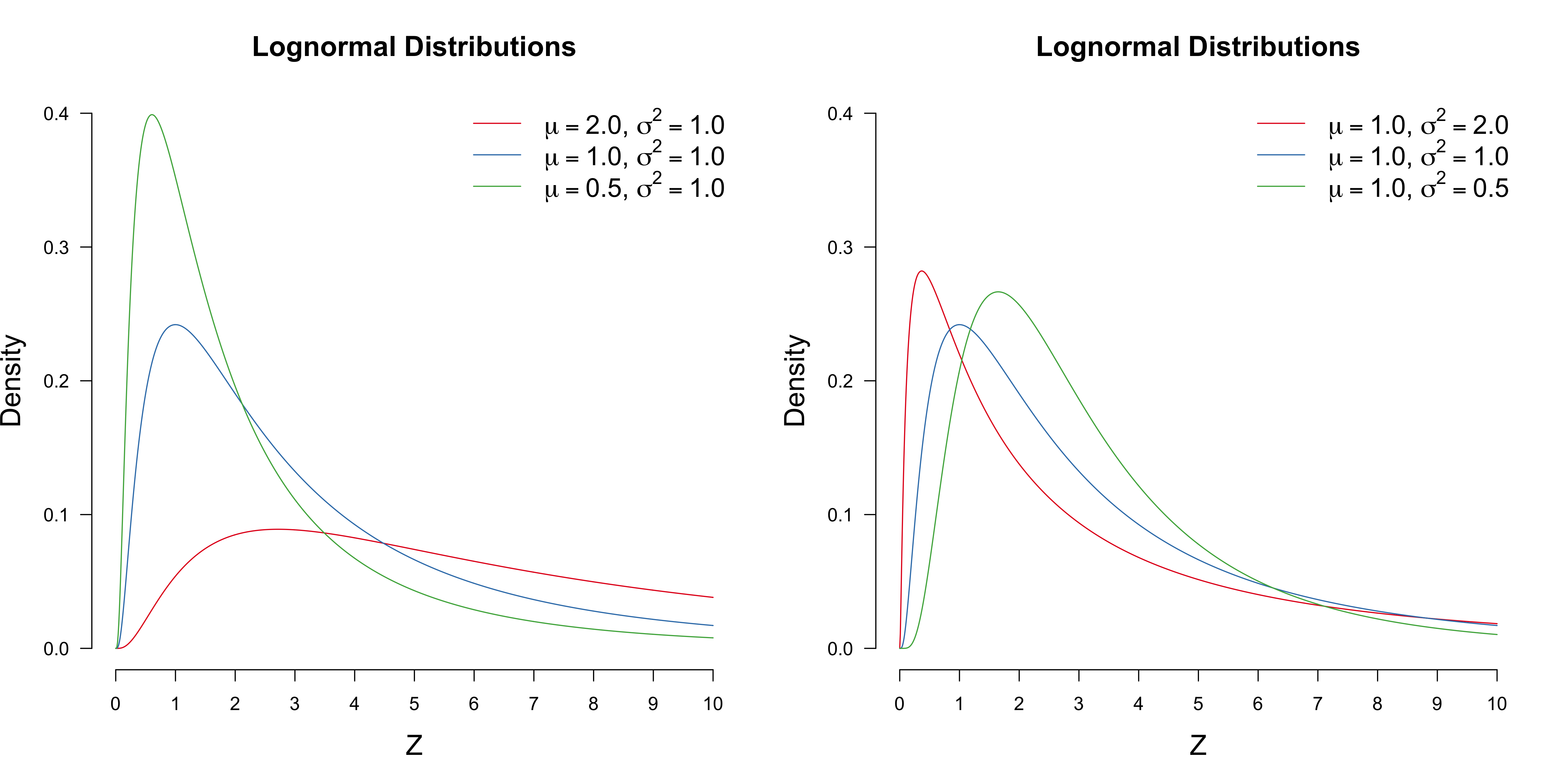
The figure below visualizes various lognormal distribution with different parameters $\mu$ and $\sigma^2$. The figure on the left shows how a change in $\sigma^2$ affects the distribution, while keeping $\mu = 1$. You can see that the “peak” of the distribution changes, indicating that the parameter $\mu$ is not independent of $\sigma^2$. In fact, while the mean and variance of a normal distribution are given by $\mu$ and $\sigma^2$, respectively, this is not so for a lognormal distribution. It seems difficult to compute the first two moments of the Lognormal distributions directly (you can try if you want!). However, there is a neat trick to compute all its moments basically instantaneously.

To do this, observe that the moment generating function (MGF) of a random variable $X$ is given by

Now, we’re not going to use the MGF of the Lognormal — in fact, because the integral diverges, it does not exist. Instead, we’ll use the MGF of a Normal distribution. Since $Z = e^X$, we can write the $t^{\text{th}}$ moment such that

where the last term is the MGF of a normal distribution (see also Blitzstein & Hwan, 2014, p. 260-261). Thus, the mean and variance of a Lognormal distribution are given by

This dependency between mean and variance is desired. In particular, it is well established that changes in mean reaction times are accompanied by proportional changes in the standard deviation (Wagenmakers & Brown, 2007).

In contrast to the Normal distribution, the Lognormal distribution is not closed under addition. This means that if $Z$ has a Lognormal distribution, $Z + \delta$ does not necessarily have a Lognormal distribution anymore. However, we are interested in modeling shifts in reaction times. For example, there is a reaction time $\alpha$ faster which participants cannot meaningfully respond. To allow for such shifts, we expand the Lognormal distribution by a parameter $\delta$ such that $Z = e^{X - \delta}$.¹⁰ This leads to the following density function

Extending the model

We extend the delayed exponential model such that

The median of a Shifted-Lognormal distribution is given by $\delta + e^\mu$, which is why we log the main part of the model above. Note that the previous asymptote $\alpha$ is now $\delta + \alpha’$. To be on the same scale as before, we assign $\delta$ and $\alpha’$ a Lognormal distribution with medians $0.50$ and $0.50$, respectively.

We can implement the model in Stan by writing a Shifted-Lognormal probability density function:

// In the function block, we define our new probability density function
 
functions {
  real shiftlognormal_lpdf(real z, real delta, real mu, real sigma) {
    real lprob;
    
    lprob = (
      -log((z - delta)*sigma*sqrt(2*pi())) -
      (log(z - delta) - mu)^2 / (2*sigma^2)
    );
    
    return lprob;
  }
  
  real shiftlognormal_rng(real delta, real mu, real sigma) {
    return delta + lognormal_rng(mu, sigma);
  }
}
 
// In the data block, we specify everything that is relevant for
// specifying the data. Note that PRIOR_ONLY is a dummy variable used later.
 
data {
  int<lower=1> n;
  real y[n];
  int<lower=0, upper=1> PRIOR_ONLY;
}
 
 
// In the parameters block, we specify all parameters we need.
// Although Stan implicitly adds flat prior on the (positive) real line
// we will specify informative priors below.
 
parameters {
  real<lower=0> r;
  real<lower=0> tau;
  real<lower=0> delta;
  real<lower=0> alpha;
  real<lower=0> beta;
  real<lower=0> sigma_e;
}
 
// In the model block, we specify our informative priors and
// the likelihood of the model, unless we want to sample only from
// the prior (i.e., if PRIOR_ONLY == 1)
 
model {
  real mu;
  // Renormalize Cauchy prior due to truncation to get correct marginal likelihood
  target += cauchy_lpdf(tau | 0, 1) - cauchy_lccdf(0 | 0, 1);
  target += lognormal_lpdf(delta | log(0.50), .5);
  target += lognormal_lpdf(alpha | log(0.50), .5);
  target += lognormal_lpdf(beta | 1, .5);
  target += gamma_lpdf(r | 1, 3);
  target += gamma_lpdf(sigma_e | 0.5, 5);
 
  if (PRIOR_ONLY == 0) {
    for (trial in 1:n) {
      mu = log(alpha + beta * (tau + 1) / (tau + exp(r*trial)));
      target += shiftlognormal_lpdf(y[trial] | delta, mu, sigma_e);
    }
  }
}
 
// In this block, we make posterior predictions (ypred) and compute
// the log likelihood of each data point given all the others (log_lik)
// which is needed for the computation of loo later
 
generated quantities {
  real mu;
  real ypred[n];
  real log_lik[n];
 
  for (trial in 1:n) {
    mu = log(alpha + beta * (tau + 1) / (tau + exp(r*trial)));
    ypred[trial] = shiftlognormal_rng(delta, mu, sigma_e);
    log_lik[trial] = shiftlognormal_lpdf(y[trial] | delta, mu, sigma_e);
  }
 
}

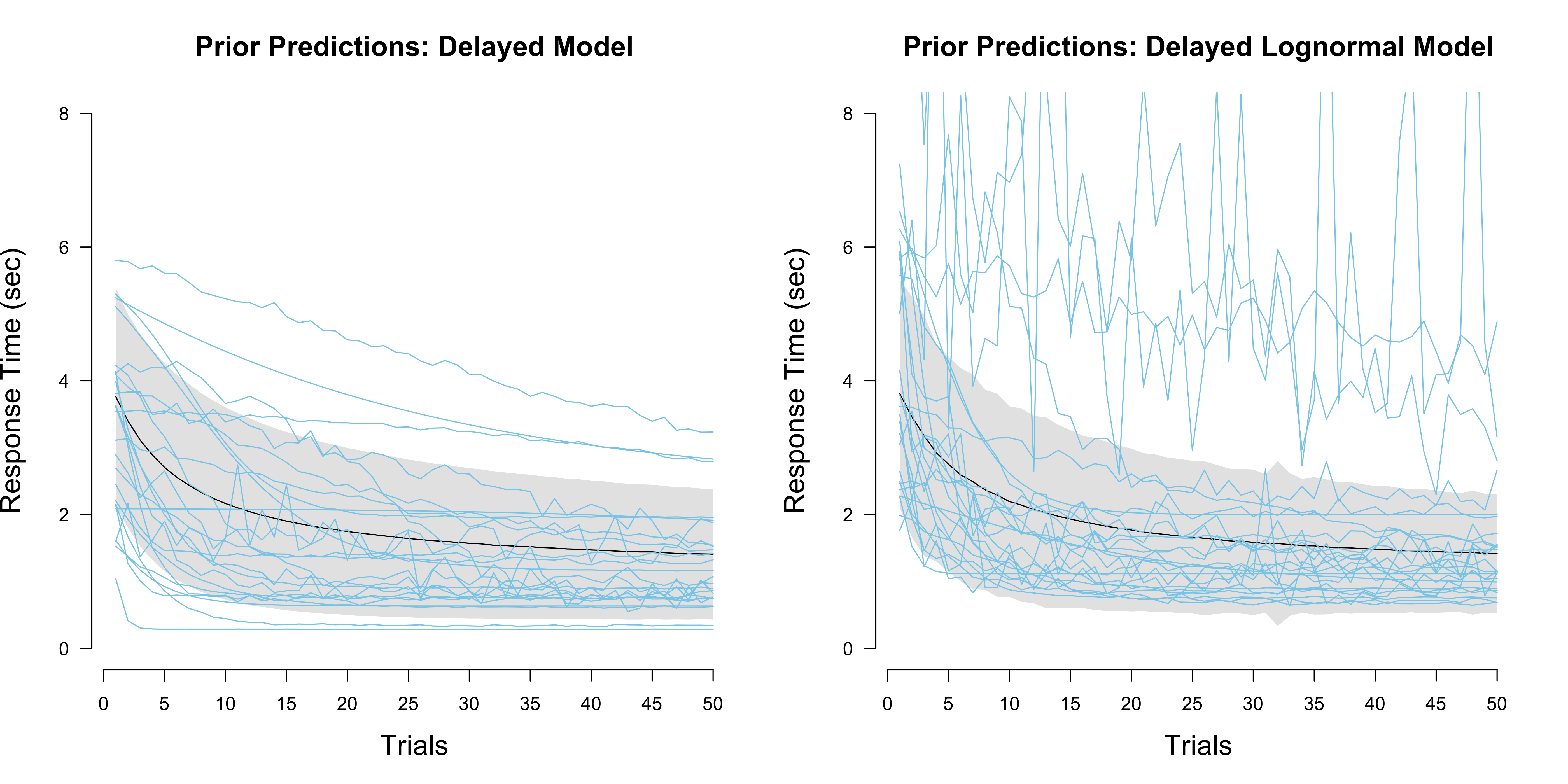
Visualizing the prior predictive distribution bares only limited insight into how these two models differ:

The Bayes factor in favour of the lognormal model is quite large:

fit_ee_plateau_lognormal <- sampling(
  comp_exp_delayed_log,
  data = list('y' = dat, 'n' = 50, 'PRIOR_ONLY' = 0),
  refresh = FALSE, chains = 4, iter = 8000, seed = 1,
  control = list(adapt_delta = 0.9)
)
 
bayes_factor(
  bridge_sampler(fit_ee_plateau_lognormal, silent = TRUE, method = 'warp3'),
  bridge_sampler(fit_ee_plateau, silent = TRUE, method = 'warp3')
)

## Estimated Bayes factor in favor of x1 over x2: 198.49106

In contrast, loo shows barely any evidence: we would not choose the lognormal model, but we remain undecided. (The warning is because we have one $k \in [0.5, 0.7]$.)

loo_compare(loo(fit_ee_plateau_lognormal), loo(fit_ee_plateau))

##        elpd_diff se_diff
## model1  0.0       0.0   
## model2 -5.1       3.3

Using stacking, the weights result in a factor of about 24 in favour of the lognormal model:

stacking_weights(fit_ee_plateau_lognormal, fit_ee_plateau)

## Method: stacking
## ------
##   weight
## 1 0.983 
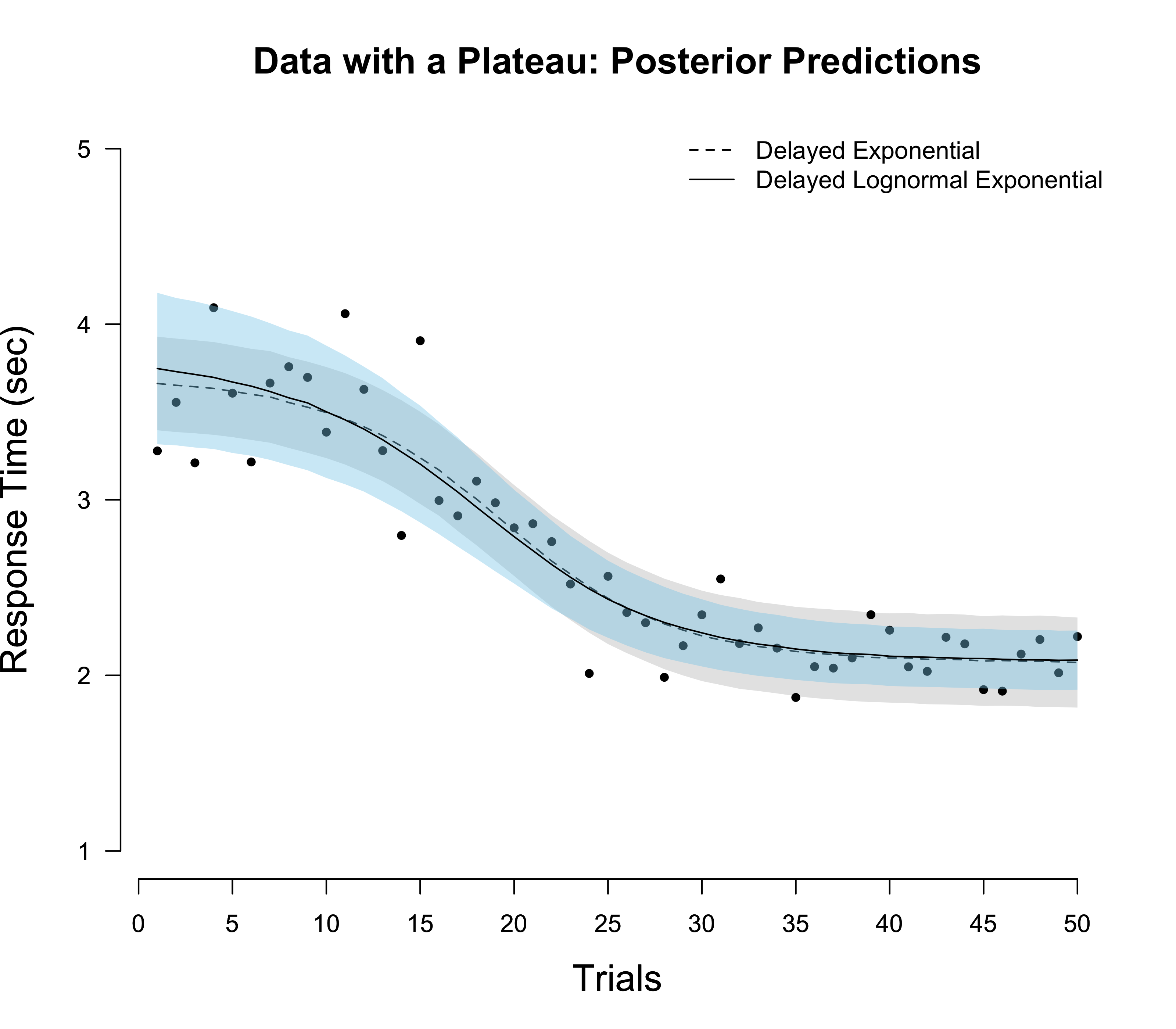
## 2 0.017

The contrast between the Bayes factor and loo can again be illuminated by looking at the posterior predictive distribution for the respective models; see below. The lognormal model can account for decrease in variance with increased practice. Still, the predictions of both models are rather similar, so that there is little to distinguish them using loo.

Modeling recap

Focusing on the exponential model, we have successively made our modeling more sophisticated (see also Evans et al., 2018). Barring priors, we have encountered the following models:

We went from (1) to (2) to account for learning plateaus; sometimes, participants take a while for learning to really kick in. We went from (2) to (3) to account for the fact that reaction times are decidedly nonnormal, and that there is a linear relationship between the mean and the standard deviation of reaction times.

We have also compared the power law to the exponential function, but so far we have looked only at simulated data. Since this blog post is already quite lengthy, we defer the treatment of real data to a future blog post.

Conclusion

In this blog post, we took a closer look at what has been dubbed the law of practice: the empirical fact that reaction time decreases as an exponential function (previously: power law) with practice. We compared two perspectives on prediction: one based on marginal likelihoods, and one based on leave-one-out cross-validation. The latter allows the model to gorge on data, update its parameters, and then make predictions based on the posterior predictive distribution, while the former forces the model to make predictions using the prior predictive distribution. We have implemented the power law and exponential model in Stan, and extended the latter to model an initial learning plateau and account for the empirical observation that not only mean reaction time decreases, but also its variance.

I would like to thank Nathan Evans, Quentin Gronau, and Don van den Bergh for helpful comments on this blog post.

References

• Blitzstein, J. K., & Hwang, J. (2014). Introduction to Probability. London, UK: Chapman and Hall/CRC.
• Evans, N. J., Brown, S. D., Mewhort, D. J., & Heathcote, A. (2018). Refining the law of practice. Psychological Review, 125(4), 592-605.
• Fong, E., & Holmes, C. (2019). On the marginal likelihood and cross-validation. arXiv preprint arXiv:1905.08737.
• Gelman, A., & Shalizi, C. R. (2013). Philosophy and the practice of Bayesian statistics. British Journal of Mathematical and Statistical Psychology, 66(1), 8-38.
• Gronau, Q. F., & Wagenmakers, E. J. (2019a). Limitations of Bayesian leave-one-out cross-validation for model selection. Computational Brain & Behavior, 2(1), 1-11.
• Gronau, Q. F., & Wagenmakers, E. J. (2019b). Rejoinder: More limitations of Bayesian leave-one-out cross-validation. Computational brain & behavior, 2(1), 35-47.
• Heathcote, A., Brown, S., & Mewhort, D. J. K. (2000). The power law repealed: The case for an exponential law of practice. Psychonomic bulletin & Review, 7(2), 185-207.
• Lee, M. D., & Vanpaemel, W. (2018). Determining informative priors for cognitive models. Psychonomic Bulletin & Review, 25(1), 114-127.
• Lee, M. D. (2018). Bayesian methods in cognitive modeling. Stevens’ Handbook of Experimental Psychology and Cognitive Neuroscience, 5, 1-48.
• Myung, I. J., Kim, C., & Pitt, M. A. (2000). Toward an explanation of the power law artifact: Insights from response surface analysis. Memory & Cognition, 28(5), 832-840.
• Newell, A. (1973). You can’t play 20 questions with nature and win: Projective comments on the papers of this symposium. In W. G. Chase (Ed.), Visual information processing (pp. 283-308). New York, US: Academic Press.
• Newell, A., & Rosenbloom, P. S. (1981). Mechanisms of skill acquisition and the law of practice. In J.R. Anderson (Ed.), Cognitive skills and their acquisition (pp. 1-55). Hillsdale, NJ: Erlbaum.
• Vehtari, A., Gelman, A., & Gabry, J. (2015). Pareto smoothed importance sampling. arXiv preprint arXiv:1507.02646.
• Vehtari, A., Simpson, D. P., Yao, Y., & Gelman, A. (2019). Limitations of “Limitations of Bayesian leave-one-out cross-validation for model selection”. Computational Brain & Behavior, 2(1), 22-27.
• Vehtari, A., Gelman, A., & Gabry, J. (2017). Practical Bayesian model evaluation using leave-one-out cross-validation and WAIC. Statistics and Computing, 27(5), 1413-1432.
• Wagenmakers, E. J., & Brown, S. (2007). On the linear relation between the mean and the standard deviation of a response time distribution. Psychological Review, 114(3), 830-841.
• Yao, Y., Vehtari, A., Simpson, D., & Gelman, A. (2018). Using stacking to average Bayesian predictive distributions (with discussion). Bayesian Analysis, 13(3), 917-1003.

Footnotes