Two perspectives on regularization

Regularization is the process of adding information to an estimation problem so as to avoid extreme estimates. Put differently, it safeguards against foolishness. Both Bayesian and frequentist methods can incorporate prior information which leads to regularized estimates, but they do so in different ways. In this blog post, I illustrate these two different perspectives on regularization on the simplest example possible — estimating the bias of a coin.

Modeling coin flips

Let’s say that we are interested in estimating the bias of a coin, which we take to be the probability of the coin showing heads.¹ In this section, we will derive the Binomial likelihood — the statistical model that we will use for modeling coin flips. Let $X \in [0, 1]$ be a discrete random variable with realization $X = x$. Flipping the coin once, let the outcome $x = 0$ correspond to tails and $x = 1$ to heads. We use the Bernoulli likelihood to connect the data to the latent parameter $\theta$, which we take to be the bias of the coin:

There is no point in estimating the bias by flipping the coin only once. We are therefore interested in a model that can account for $n$ coin flips. If we are willing to assume that the individual coin flips are independent and identically distributed conditional on $\theta$, we can obtain the joint probability of all outcomes by multiplying the probability of the individual outcomes:

For the purposes of estimating the coin’s bias, we actually do not care about the order in which the coins come up heads or tails; we only care about how frequently the coin shows heads or tails out of $n$ throws. Thus, we do not model the individual outcomes $X_i$, but instead model their sum $Y = \sum_{i=1}^n X_i$. We write:

where we suppress conditioning on $n$ to not clutter notation. Note that our model is not complete — we need to account for the fact that there are several ways to get $y$ heads out of $n$ throws. For example, we can get $y = 2$ with $n = 3$ in three different ways: $(1, 1, 0)$, $(0, 1, 1)$, and $(1, 0, 1)$. If we were to use the model above, we would underestimate the probability of observing two heads out of three coin tosses by a factor of three.

In general, there are $n!$ possible ways in which we can order the outcomes. To see this, think of $n$ containers. The first outcome can go in any container, the second one in any container but the container which houses the first outcome, and so on, which yields:

However, we only care about $y$ of them, so we need to remove the remaining $(n - y)!$ possible ways. Moreover, once we have taken $y$ outcomes, we do not care about their order; thus we remove another $y!$ permutations. Therefore, for any particular sequence of coin flips of length $n$, there are

ways to get $y$ heads out of $n$ throws. The funny looking symbol on the right is the Binomal coefficient. The probability of the data is therefore given by the Binomial likelihood:

which just adds the term ${n \choose y}$ to the equation we had above after introducing $Y$. For the example of observing $y = 2$ heads out of $n = 3$ coin flips, the Binomial coefficient is ${3 \choose 2} = 3$, which accounts for the fact that there are three possible ways to get two heads out of three throws.

The data

Assume we flip the coin three times, $n = 3$, and observe three heads, $y = 3$. How can we estimate the bias of the coin? In the next sections, we will use the Binomial likelihood derived above and discuss three different ways of estimating the coin’s bias: maximum likelihood estimation, Bayesian estimation, and penalized maximum likelihood estimation.

Classical estimation

Within the frequentist paradigm, the method of maximum likelihood is arguably the most popular method for parameter estimation: choose as an estimate for $\theta$ the value which maximizes the likelihood of the data.² To get a feeling for how the likelihood of the data differs across values of $\theta$, let’s pick two values, $\theta_1 = .5$ and $\theta_2 = 1$, and compute the likelihood of observing three heads out of three coin flips:

We therefore conclude that the data are more likely for a coin that has bias $\theta_1 = 1$ than for a coin that has bias $\theta_2 = 0.5$. But is it the most likely value? To compare all possible values for $\theta$ visually, we plot the likelihood as a function of $\theta$ below. The left figure shows that, indeed, $\theta = 1$ maximizes the likelihood for the data. The right figure shows the likelihood function for $y = 15$ heads out of $n = 20$ coin flips. Note that, in contrast to probabilities, which need to sum to one, likelihoods do not have a natural scale.

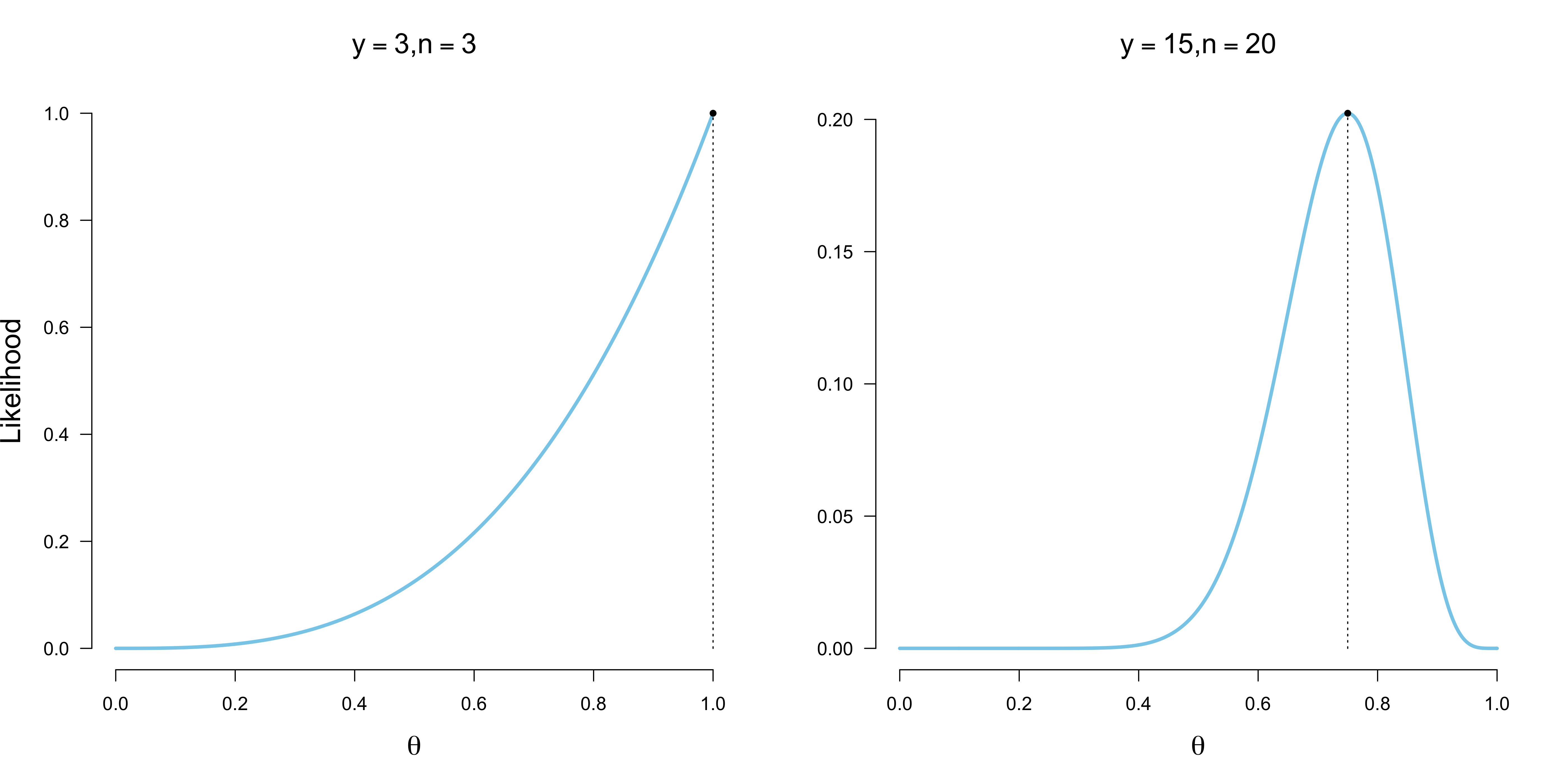
Do these two examples allow us to derive a general principle for how to estimate the bias of a coin? Let $\hat{\theta}$ denote an estimate of the population parameter $\theta$. The two figures above suggests that $\hat{\theta} = \frac{y}{n}$ is the maximum likelihood estimate for an arbitrary data set $d = (y, n)$ … and it is! To arrive at this mathematically, we can find the maximum of this likelihood function by taking the derivative with respect to $\theta$, and setting it to zero (see also a previous post). In other words, we solve for the value of $\theta$ for which the derivative does not change; and since the Binomial likelihood is unimodal, this maximum will be unique. Note the value for $\theta$ at which the likelihood function has its maximum does not change when we take logs, but because the mathematics is greatly simplified, we do so:

which shows that indeed $\frac{y}{n}$ is the maximum likelihood estimate.

Bayesian estimation

Bayesians assign priors to parameters in addition to the likelihood, which takes a central role in all statistical paradigms. For this Binomial problem, we assign $\theta$ a Beta prior:

As we will see below, this prior allows easy Bayesian updating while being sufficiently flexible in incorporating prior information. The figure below shows different Beta distributions, formalizing our prior belief about values of $\theta$.

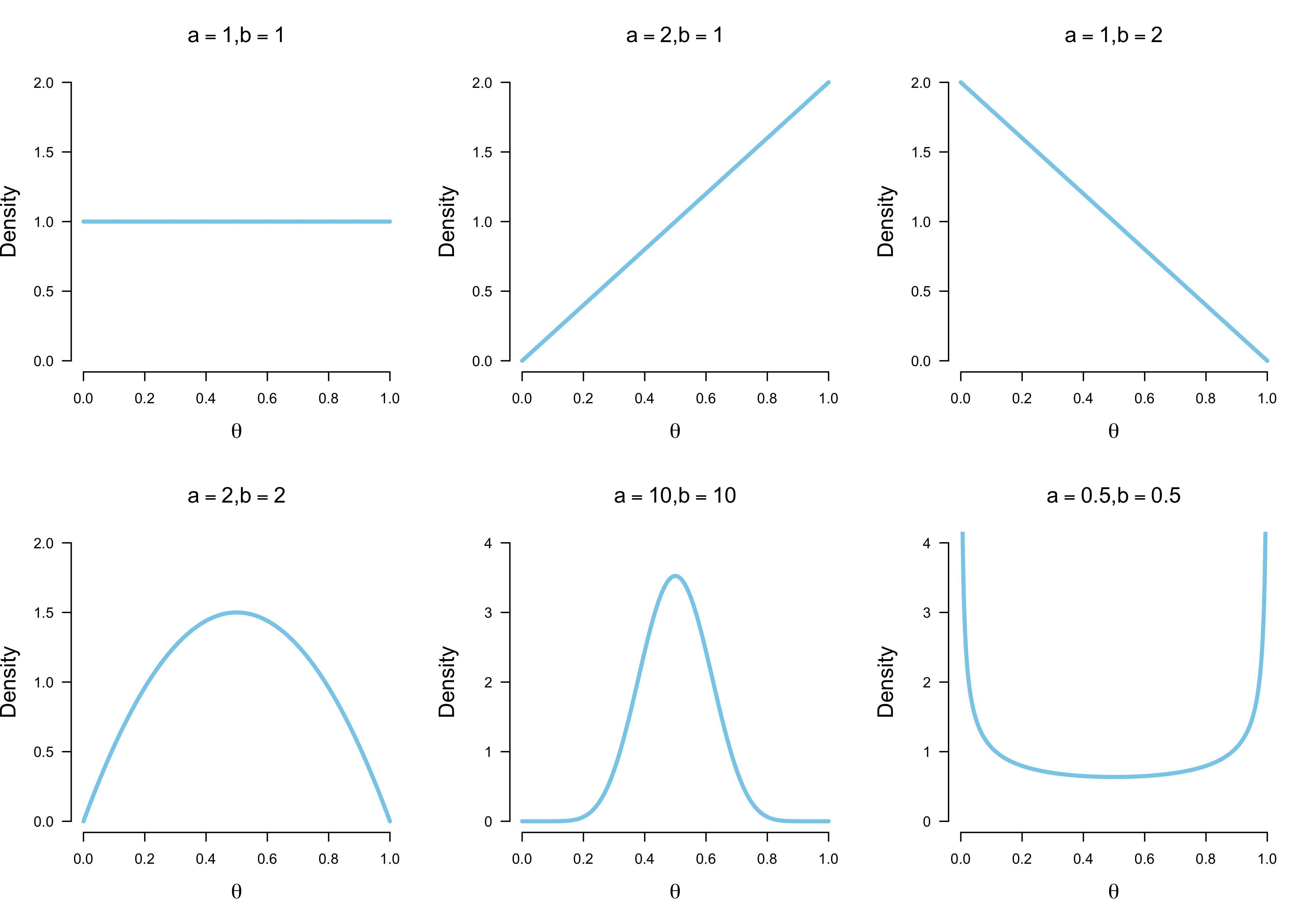
The figure in the top left corner assigns uniform prior plausibility to all values of $\theta$; the figures to its right incorporate a slight bias towards the extreme values $\theta = 1$ and $\theta = 0$. With increasing $a$ and $b,$ the prior becomes more biased towards $\theta = 0.5$; with decreasing $a$ and $b$, the prior becomes biased against $\theta = 0.5$.

As shown in a previous blog post, the Beta distribution is conjugate to the Binomial likelihood, which means that the posterior distribution of $\theta$ is again a Beta distribution:

where $a’ = a + y$ and $b’ = b + n - y$. Under this conjugate setup, the parameters of the prior can be understood as prior data; for example, if we choose prior parameters $a = b = 1$, then we assume that we have seen one heads and one tails prior to data collection. The figure below shows two examples of such Bayesian updating processes.

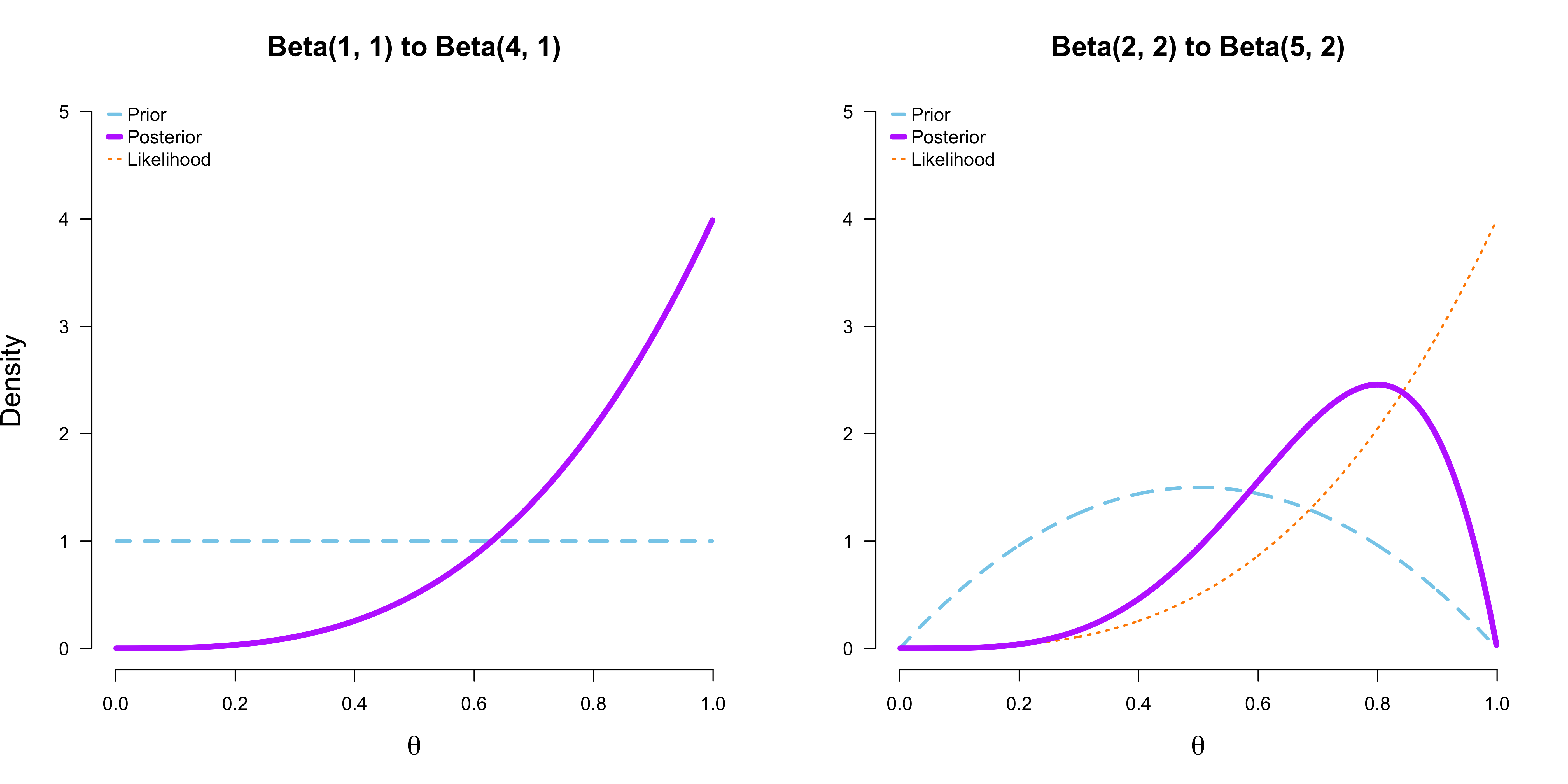
In both cases, we observe $y = 3$ heads out of $n = 3$ coin flips. On the left, we assign $\theta$ a uniform prior. The resulting posterior distribution is proportional to the likelihood (which we have rescaled to fit nicely in the graph) and thus does not appear as a separate line. After we have seen the data, we can compute the posterior mode as our estimate for the most likely value of $\theta$. Observe that the posterior mode is equivalent to the maximum likelihood estimate:

This is in fact the case for all statistical estimation problems where we assign a uniform prior to the (possibly high-dimensional) parameter vector $\theta$. To prove this, observe that:

since we can drop the normalizing constant $p(y)$, because it does not depend on $\theta$, and $p(\theta)$, because it is a constant assigning all values of $\theta$ equal probability.

Using a Beta prior with $a = b = 2$, as shown on the right side of the figure above, we see that the posterior is not proportional to the likelihood anymore. This in turn means that the mode of the posterior distribution does no longer correspond to the maximum likelihood estimate. In this case, the posterior mode is:

In contrast to earlier, this estimate is shrunk towards $\theta = 0.5$. This came about because we have used prior information that stated that $\theta = 0.5$ is more likely than the other values (see figure with $a = b = 2$ above). Consequently, we were therefore less swayed by the somewhat unlikely situation (under no bias $\theta = 0.5$) of observing three heads out of three throws. It should thus not come as a surprise that Bayesian priors can act as regularizing devices. However, this requires careful application, especially in small sample size settings.

In a Post Scriptum to this blog post, I similarly show how the posterior mean, which is arguably are more natural point estimate as it takes the uncertainty about $\theta$ better into account than the posterior mode, can be viewed as a regularized estimate, too.

Penalized estimation

Bayesians are not the only ones who can add prior information to an estimation problem. Within the frequentist framework, penalized estimation methods add a penalty term to the log likelihood function, and then find the parameter value which maximizes this penalized log likelihood. We can implement such a method by optimizing an extended log likelihood:

where we penalize values that a far from the parameter value which indicates no bias, $\theta = 0.5$. The larger $\lambda$, the stronger values of $\theta \neq 0.5$ get penalized. In addition to picking $\lambda$, the particular form of the penalty term is also important. Similar to assigning $\theta$ a prior distribution, although possibly less straightforward and less flexible, choosing the penalty term means incorporating information about the problem in addition to specifying a likelihood function. Above, we have used the squared distance from $\theta = 0.5$ as a penalty. We call this the $\mathcal{L}_2$-norm penalty³, but the $\mathcal{L}_1$-norm, which takes the absolute distance, is an equally interesting choice:

As we will see below, these penalties have very different effects.

The penalized likelihood does not only depend on $\theta$, but also on $\lambda$. The code below evaluates the penalized log likelihood function given values for these two parameters. Note that we drop the normalizing constant ${n \choose y}$ as it does neither depend on $\theta$ nor on $\lambda$.

fn <- function(y, n, theta = seq(0.001, .999, .001), lambda = 2, reg = 1) {
  y * log(theta) + (n - y) * log(1 - theta) - lambda * abs(theta - 1/2)^reg
}
 
get_penalized_likelihood <- Vectorize(fn)

With only three data points it is futile to try to estimate $\lambda$ using, for example, cross-validation; however, this is also not the goal of this blog post. Instead, to get further intuition, we simply try out a number of values for $\lambda$ using the code below and see how it influences our estimate of $\theta$. Because the parameter space has only one dimension, we can easily find the value for $\theta$ which maximizes the penalized likelihood even without wearing our calculus hat. Specifically, given a particular value for $\lambda$, we evaluate the penalized likelihood function for a range of values of between zero and one and pick the value that minimizes it.

estimate_path <- function(y, n, reg = 1) {
  lambda_seq <- seq(0, 10, .01)
  theta_seq <- seq(.001, 1, .001)
  
  theta_best <- sapply(seq_along(lambda_seq), function(i) {
    penalized_likelihood <- get_penalized_likelihood(y, n, theta_seq, lambda_seq[i], reg)
    theta_seq[which.max(penalized_likelihood)]
  })
  
  cbind(lambda_seq, theta_best)
}

Sticking with the observations of three heads ($y = 3$) out of three throws ($n = 3$), the figure below plots best fitting values for $\theta$ given a range of values for $\lambda$. Observe that the $\mathcal{L}_1$-norm penalty shrinks it more quicker and abruptly to $\theta = 0.5$ at $\lambda = 6$, while the $\mathcal{L}_2$-norm penalty gradually (and rather slowly) shrinks the parameter to $\theta = 0.5$ with increasing $\lambda$. Why is this so?

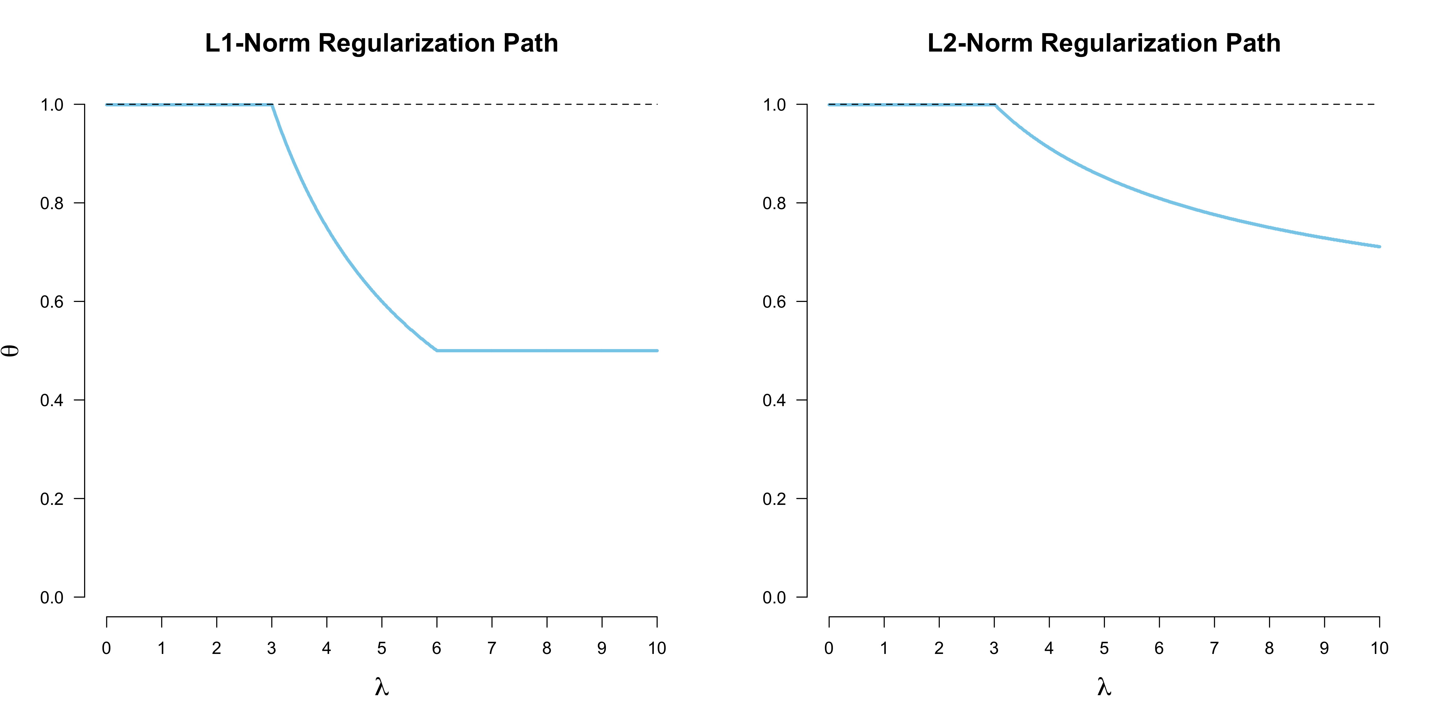
First, note that because $\theta \in [0, 1]$ the squared distance will always be smaller than the absolute distance, which explains the slower shrinkage. Second, the fact that the $\mathcal{L}_1$-norm penalty can shrink exactly to $\theta = 0.5$ is due to the discontinuity of the absolute value function. The figures below provides some intuition. In particular, the figure on the left shows the $\mathcal{L}_1$-norm penalized likelihood function for a select number of $\lambda$’s. We see that for $\lambda < 3$, the value $\theta = 1$ performs best. With $\lambda \in [3, 6]$, values of $\theta \in [0.5, 1]$ become more likely than the extreme estimate $\theta = 1$. For $\lambda \geq 6$, the ‘no bias’ value $\theta = 0.5$ maximizes the penalized likelihood. Due to the discontinuity in the penalty, the shrinkage is exact. The $\mathcal{L}_2$-norm penalty, on the other hand, shrinks less strongly, and never exactly to $\theta = 0.5$, except of course for $\lambda \rightarrow \infty$. We can see this in the right figure below, where the penalized likelihood function is merely shifted to the left with increasing $\lambda$; this is in contrast to the $\mathcal{L}_1$-norm penalized likelihood on the left, for which the value $\theta = 0.5$ at the discontinuity takes a special place.

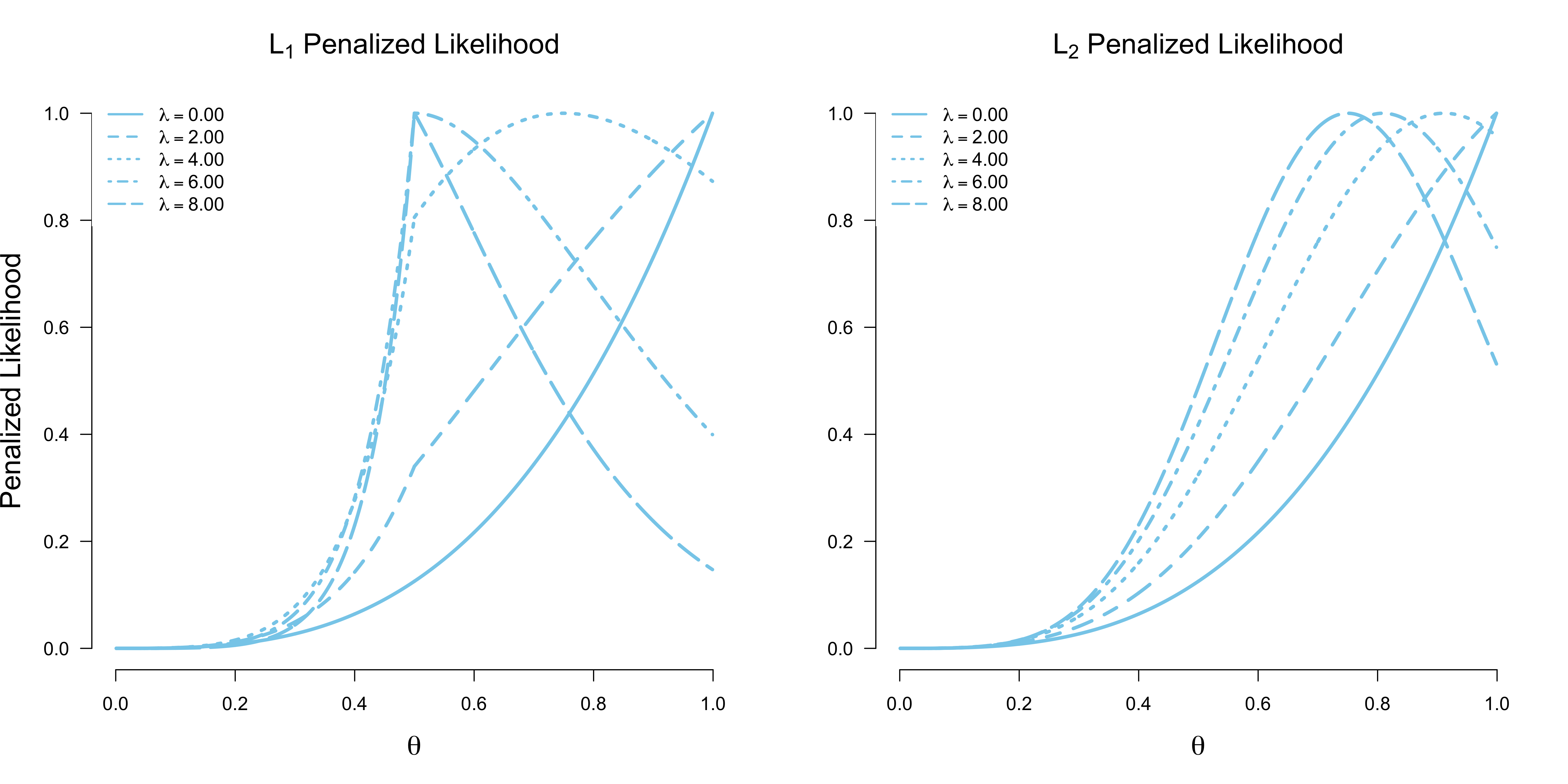
You can play around with the code below to get an intuition for how different values of $\lambda$ influence the penalized likelihood function.

library('latex2exp')
 
plot_pen_llh <- function(y, n, lambdas, reg = 1,
                         ylab = 'Penalized Likelihood', title = '') {
  
  nl <- length(lambdas)
  theta <- seq(.001, .999, .001)
  
  likelihood <- matrix(NA, nrow = nl, ncol = length(theta))
  normalize <- function(x) (x - min(x)) / (max(x) - min(x))
  
  for (i in seq(nl)) {
    log_likelihood <- get_penalized_likelihood(y, n, theta, lambdas[i], reg)
    likelihood[i, ] <- normalize(exp(log_likelihood))
  }
  
  plot(theta, likelihood[1, ], xlim = c(0, 1), type = 'l', ylab = ylab, lty = 1,
       xlab = TeX('$\\theta$'), main = title, lwd = 3, cex.lab = 1.5,
       cex.main = 1.5, col = 'skyblue', axes = FALSE)
       
  for (i in seq(2, nl)) {
    lines(theta, likelihood[i, ], xlim = c(0, 1), type = 'l', ylab = ylab, lty = i,
          lwd = 3, cex.lab = 1.5, cex.main = 1.5, col = 'skyblue')
  }
  
  axis(1, at = seq(0, 1, .2))
  axis(2, las = 1)
  
  info <- sapply(lambdas, function(l) TeX(sprintf('$\\lambda = %.2f$', l)))
  legend('topleft', legend = info, lty = seq(nl), cex = 1,
         box.lty = 0, col = 'skyblue', lwd = 2)
}
 
lambdas <- c(0, 2, 4, 6, 8)
plot_pen_llh(3, 3, lambdas, reg = 1, title = TeX('$L_1$ Penalized Likelihood'))
plot_pen_llh(3, 3, lambdas, reg = 2, title = TeX('$L_2$ Penalized Likelihood'))

In practice, one would reparameterize this model as a logistic regression, and use cross-validation to estimate the best value for $\lambda$; see the Post Scriptum for a sketch of this approach.

Conclusion

In this blog post, we have seen two perspectives regularization illustrated on a very simple example: estimating the bias of a coin. We first derived the Binomial likelihood, connecting the data to a parameter $\theta$ which we took to be the bias of the coin, as well as the maximum likelihood estimate. Observing three heads out of three coin flips, we became slightly uncomfortable with the (extreme) estimate $\hat{\theta} = 1$. We have seen how, from a Bayesian perspective, one can add prior information to this estimation problem, and how this led to an estimate that was shrunk towards $\theta = 0.5$. Within the frequentist framework, one can add information by augmenting the likelihood function with a penalty term. The type of information we want to incorporate corresponds to the particular penalty term. In this blog post, we have focused on the most commonly used penalty terms: the $\mathcal{L}_1$-norm, which shrinks parameters exactly to a particular value; and the $\mathcal{L}_2$-norm penalty, which provides continuous shrinkage. A future blog post might look into linear regression models where regularization methods abound and study how, for example, the popular Lasso can be recast in Bayesian terms.

I would like to thank Jonas Haslbeck, Don van den Bergh, and Sophia Crüwell for helpful comments on this blog post.

Post Scriptum

Posterior mean

You may argue that one should use the mean instead of the mode as a posterior summary measure. If one does this, then there is already some shrinkage for the case of uniform priors. The mean of the posterior distribution is given by:

As so often in mathematics, we can rewrite this in a more complicated manner to gain insight into how Bayesian priors shrink estimates:

This decomposition shows that the posterior mean is a weighted combination of the prior mean and the maximum likelihood estimate. Since we can think of $a + b$ as the prior data, note that $a + b + n$ can be thought of as the total number of data points. The prior mean is thus weighted be the proportion of prior to total data, while the maximum likelihood estimate is weighted by the proportion of sample data to total data. This provides another perspective on how Bayesian priors regularize estimates.⁴

Penalized logistic regression

Cross-validation might be a bit awkward when we represent the data using only $y$ and $n$. We can go back to the product of Bernoulli representation, which uses all individual data points $x_i$. This results in a logistic regression problem with likelihood:

where we use a sigmoid function as the link function, and $\beta$ is on the log odds scale. The penalized log likelihood function can be written as

where because $\beta = 0$ corresponds to $\theta = 0.5$, we do not need to subtract in the penalty term. This parameterization also makes it more easy to study which types of priors on $\beta$ result in an $\mathcal{L}_1$ or $\mathcal{L}_2$ norm penalty (spoiler: it’s a Laplace and the Gaussian, respectively). Such models can be estimated using the R package glmnet, although it does not work for the exceedingly small sample we have played with in this blog post. This seems to imply that regularization is more natural in the Bayesian framework, which additionally allows more flexible specification of prior knowledge.

References

• Gelman, A., & Nolan, D. (2002). You can load a die, but you can’t bias a coin. The American Statistician, 56(4), 308-311.
• Stigler, S. M. (2007). The Epic Story of Maximum Likelihood. Statistical Science, 22(4), 598-620.

Footnotes