A gentle introduction to dynamical systems theory

Dynamical systems theory provides a unifying framework for studying how systems as disparate as the climate and the behaviour of humans change over time. In this blog post, I provide an introduction to some of its core concepts. Since the study of dynamical systems is vast, I will barely scratch the surface, focusing on low-dimensional systems that, while rather simple, nonetheless show interesting properties such as multiple stable states, critical transitions, hysteresis, and critical slowing down.

While I have previously written about linear differential equations (in the context of love affairs) and nonlinear differential equations (in the context of infectious diseases), this post provides a gentler introduction. If you have not been exposed to dynamical systems theory before, you may find this blog post more accessible than the other two.

The bulk of this blog post may be read as a preamble to Dablander, Pichler, Cika, & Bacilieri (2020), who provide an in-depth discussion of early warning signals and critical transitions. I recently gave a talk on this work and had the chutzpah to have it be recorded (with slides available from here). The first thirty minutes or so cover part of what is explained here, in case you prefer frantic hand movements to the calming written word. But without any further ado, let’s dive in!

Differential equations

Dynamical systems are systems that change over time. The dominant way of modeling how such systems change is by means of differential equations. Differential equations relate the rate of change of a quantity $x$ — which is given by the time derivative $\frac{\mathrm{d}x}{\mathrm{d}t}$ — to the quantity itself:

If we knew the function $f$, then this differential equation would give us the rate of change for any value of $x$. We are not particularly interested in this rate of change per se, however, but at the value of $x$ as a function of time $t$. We call the function $x(t)$ the solution of the differential equation. Most differential equations cannot be solved analytically, that is, we cannot get a closed-form expression of $x(t)$. Instead, differential equations are frequently solved numerically.

How the system changes as a function of time, given by $x(t)$, is implicitly encoded in the differential equation. This is because, given any particular value of $x$, $f(x)$ tells us in which direction $x$ will change, and how quickly. It is this fact that we exploit when numerically solving differential equations. Specifically, given an initial condition $x_0 \equiv x(t = 0)$, $f(x_0)$ tells us in which direction and how quickly the system is changing. This suggests the following approximation method:

where $n$ indexes the set {$x_0, x_1, \ldots$} and $\Delta_t$ is the time that passes between two iterations. This is the most primitive way of numerically solving differential equations, known as Euler’s method, but it will do for this blog post. The derivative $\frac{\mathrm{d}x}{\mathrm{d}t}$ tells us how $x$ changes in an infinitesimally small time interval $\Delta_t$, and so for sufficiently small $\Delta_t$ we can get a good approximation of $x(t)$. In computer code, Euler’s method looks something like this:

solve <- function(f, x0, delta_t = 0.01, nr_iter = 1000) {
  
  xt <- rep(x0, nr_iter)
  
  for (n in seq(2, nr_iter + 1)) {
    xt[n] <- xt[n-1] + delta_t * f(xt[n-1])
  }
  
  time <- seq(0, nr_iter * delta_t, delta_t)
  res <- cbind(time, xt)
  res
}

The equation above is a deterministic differential equation — randomness does not enter the picture. If one knows the initial condition, then one can perfectly predict the state of the system at any time point $t$.¹ In the next few sections, we use simple differential equations to model how a population grows over time.

Modeling population growth

Relatively simple differential equations can lead to surprisingly intricate behaviour. Over the next few sections, we will discover this by slowly extending a simple model for population growth.

Exponential growth

In his 1798 Essay on the Principle of Population, Thomas Malthus noted the problems that may come about when the growth of a population is proportional to its size.² Letting $N$ be the number of individuals in a population, we may formalize such a growth process as:

which states that the change in population size is proportional to itself, with $r > 0$ being a parameter indicating the growth rate. Using $r = 1$, the left panel in the figure below visualizes this linear differential equation. The right panel visualizes its solutions, that is, the number of individuals as a function of time, $N(t)$, for three different initial conditions.

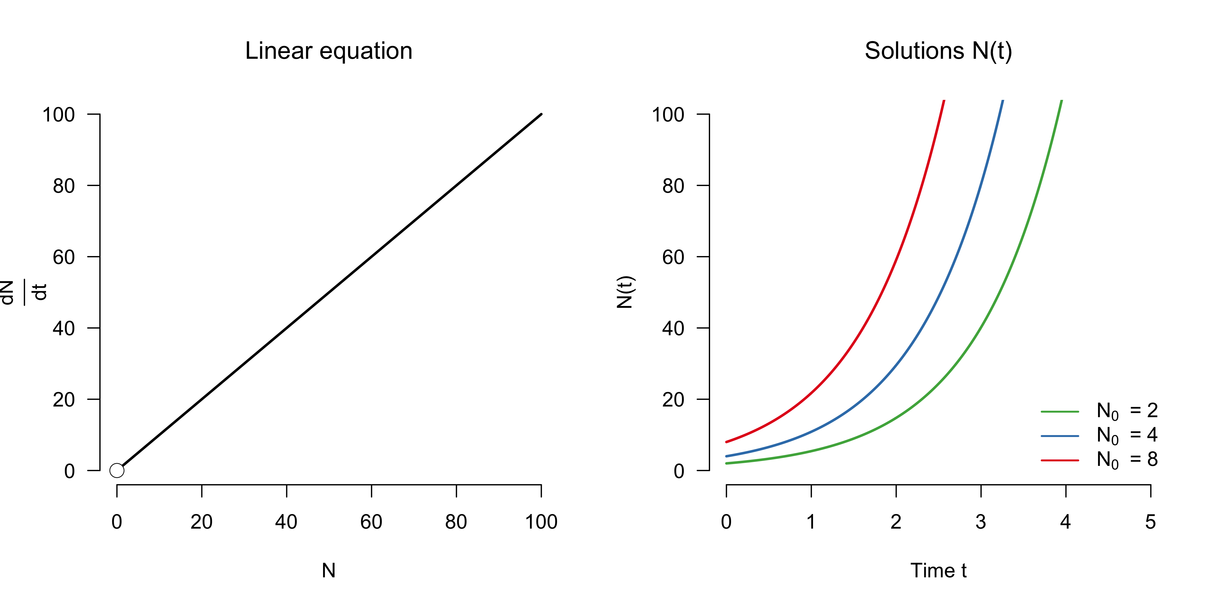
As can be seen, the population grows exponentially, without limits. While differential equations cannot be solved analytically in general, linear differential equations can. In our case, the solution is given by $N(t) = N_0 e^{t}$, as derived in a previous blog post.

You can reproduce the trajectories shown in the right panel by using our solver from above:

malthus <- function(x) x
solution_malthus <- solve(f = malthus, x0 = 2, nr_iter = 500, delta_t = 0.01)

We can inquire about qualitative features of dynamical systems models. One key feature are equilibrium points, that is, points at which the system does not change. Denote such points as $N^{\star}$, then formally:

In our model, the only equilibrium point is $N = 0$. Equilibrium points — also called fixed points — can be stable or unstable. A system that is at a stable equilibrium point returns to it after a small, exogeneous perturbation, but does not do so at an unstable equilibrium point. $N = 0$ is an unstable equilibrium point, and this is indicated by the white circle in the left panel above. In other words, if the population size is zero, and if we were to add some individuals, then the population would grow exponentially rather than die out.

Units and time scales

In a differential equation, the units of the left hand-side must match the units of the right-hand side. In our example above, the left hand-side is given in population per unit of time, and so the right hand-side must also be in population per unit of time. Since $N$ is given in population, $r$ must be a rate, that is, have units $1 / \text{time}$. This brings us to a key question when dealing with dynamical system models. What is the time scale of the system?

The model cannot by itself provide an appropriate time scale. In our case, it clearly depends on whether we are looking at, say, a population of bacteria or rabbits. We can provide the system with a time scale by appropriately changing $r$. Take the bacterium Escherichia coli, which can double every 20 minutes. We know from above that this means exponential growth:

Supposing that we start with two bacteria $N_0 = 2$, then the value of $r$ that leads to a doubling every twenty minutes is given by:

where this growth rate is with respect to twenty minutes. To get this per minute, we write $r_{\text{coli}} = \text{log }2 / 20$, resulting in the following differential equation for the population growth of Escherichia coli:

where the unit of time is now minutes. What about a population of rabbits? They grow much slower, of course. Suppose they take three months to double in population size (but see here). This also yields a rate $r_{\text{rabbits}} = \text{log }2$, but this is with respect to three months. To get this in minutes, we assume that one month has 30 days and write

This yields the following differential equation for the growth of a population of rabbits:

The figure below contrasts the growth of Escherichia coli (left panel) with the growth of rabbits (right panel). Unsurprisingly, we see that rabbits are much slower — compare the $x$-axes! — to increase in population than Escherichia coli.³

This exponential growth model assumes that populations grow indefinitely, without limits. This is arguably incorrect, as Pierre-François Verhulst, a Belgian number theorist, was quick to point out.

Sigmoidal population growth

A population cannot grow indefinitely because its growth depends on resources, which are finite. To account for this, Pierre-François Verhulst introduced a model with a carrying capacity K in 1838, which gives the maximum size of the population that can be sustained given resource constraints (e.g., Bacaër, 2011, pp. 35-39). He wrote:

This equation is nonlinear in $N$ and is known as the logistic equation. If $K > N$ then $(1 − N / K) < 1$, slowing down the growth rate of $N$. If on the other hand $N > K$, then the population needs more resources than are available, and the growth rate becomes negative, resulting in population decrease.

The equation above has particular units. For example, $N$ gives the number of individuals in a population, be it bacteria or rabbits, and $K$ counts the maximum number of individuals that can be sustained given the available resources. Similarly, $r$ is a rate with respect to minutes or months, for example. For the purposes of this blog post, we are interested in general properties of this system and extensions thereof, rather than in modeling any particular real-world system. Therefore, we want to get rid of the parameters $K$ and $r$, which are specific to a particular population (say bacteria or rabbits).

We can eliminate $K$ by reformulating the differential equation in terms of $x = \frac{N}{K}$, which is $1$ if the population is at the carrying capacity. Implicit differentiation yields $K \cdot \mathrm{d}x = \mathrm{d}N$, which when plugged into the system gives:

Both $N$ and $K$ count the number of individuals (e.g., bacteria or rabbits) in the population, and their ratio $x$ is unit- or dimensionless. For example, $x = 0.50$ means that the population is at half the size that can be sustained at carrying capacity, and we do not need to know the exact number of individuals $N$ and $K$ for this statement to make sense.

In other words, we have non-dimensionalized the differential equation, at least in terms of $x$. We can also remove the dimension of time (whether it is minutes or months, for example), by making the change of variables $\tau = t r$. Since $t$ is given in units of time, and $r$ is given in inverse units of time since it is a rate, $\tau$ is dimensionless. Implicit differentiation yields $\frac{1}{r}\mathrm{d}\tau = \mathrm{d}t$, which plugged in gives:

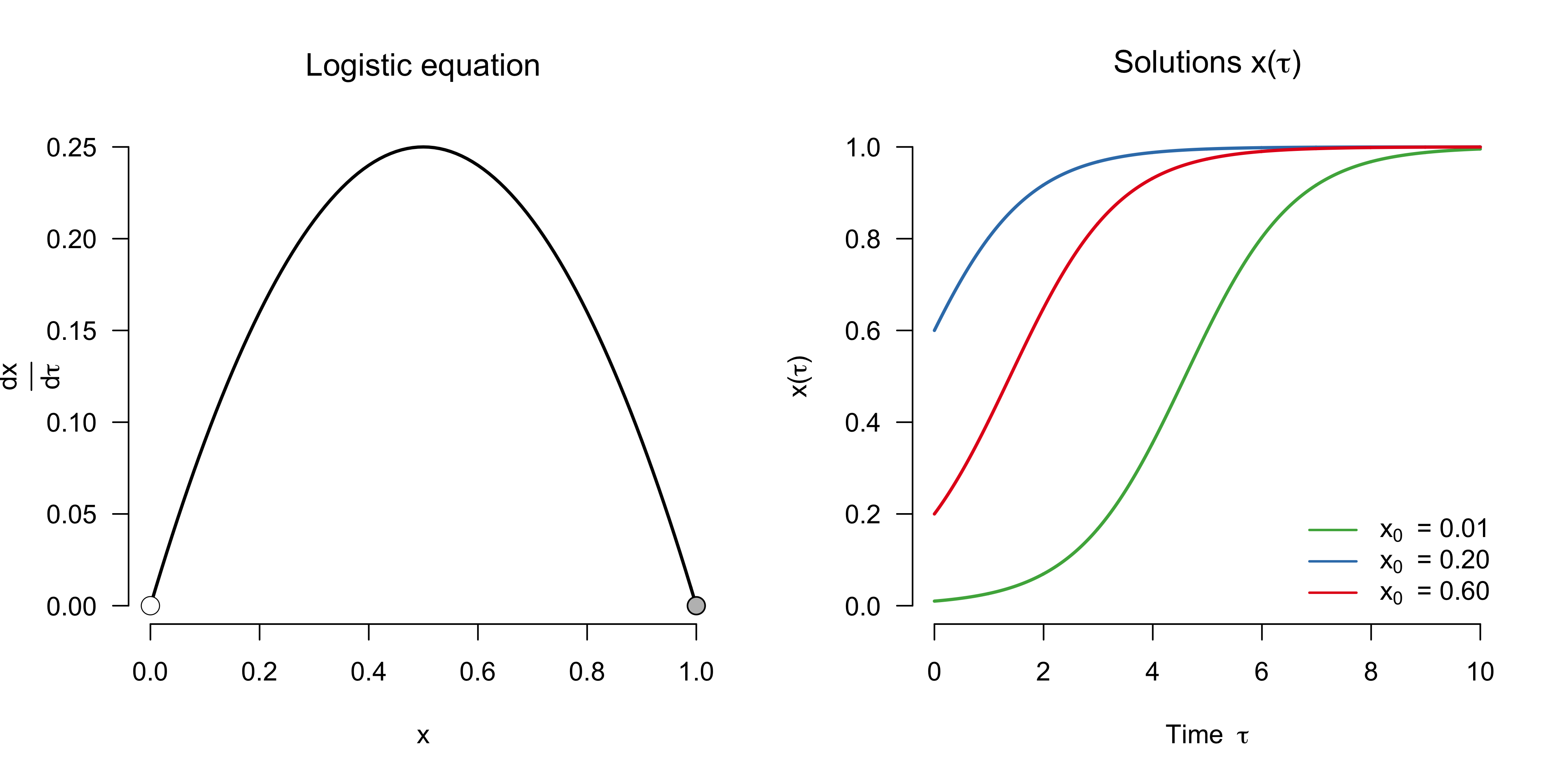
This got rid of another parameter, $r$, and hence simplifies subsequent analysis. The differential equation now tells us how the population relative to carrying capacity ($x$) changes per unit of dimensionless time ($\tau$). The left panel below shows the dimensionless logistic equation, while the right panel shows its solution for three different initial conditions.⁴

You can again reproduce the solutions by running:

verhulst <- function(x) x * (1 - x)
solution_verhulst <- solve(f = verhulst, x0 = 0.01, nr_iter = 1000, delta_t = 0.01)

In contrast to the exponential population growth in the previous model, this model shows a sigmoidal growth that hits its ceiling at carrying capacity, $x = N / K = 1$.

We can again analyze the equilibrium points of this system. In addition to the unstable fixed point at $x^{\star} = 0$, the model also has a stable fixed point at $x^{\star} = N / K = 1$, which is indicated by the gray circle in the left panel. Why is this point stable? Looking at the left panel above, we see that if we were to decrease the population size we have that $\frac{\mathrm{d}x}{\mathrm{d}\tau} > 0$, and hence the population increases towards $x^{\star} = 1$. If, on the other hand, we would increase the population size above the carrying capacity $x > 1$, we have that $\frac{\mathrm{d}x}{\mathrm{d}\tau} < 0$ (not shown in the graph), and so the population size decreases towards $x^{\star} = 1$.

Given any initial condition $x_0 > 0$, the system moves towards the stable equilibrium point $x^{\star} = 1$. This initial movement is a transient phase. Once this phase is over, the system stays at the stable fixed point forever (unless perturbations move it away). I will come back to transients in a later section.

While we have improved on the exponential growth model by encoding limits to growth, many populations are subject to another force that constraints their growth: predation. In the next section, we will extend the model to allow for predation.

Population growth under predation

In a classic article, Robert May (1977) studied the following model:

which includes a predation term that depends nonlinearly on the population size $x$.⁵ This term tells us, for any population size $x$, how strong the pressure on the population due to predation is. The parameter $\alpha$ gives the saturation point, that is, the population size at which predation slows down. If this value is low, the extent of predation rises rapidly with an increased population. To see this, the left panel in the figure below visualizes the predation term for different values of $\alpha$, fixing $\gamma = 0.50$. The parameter $\gamma$, on the other hand, influences the maximal extent of predation. Fixing $\alpha = 0.10$, the right panel shows how the extent of the predation increases with $\gamma$.

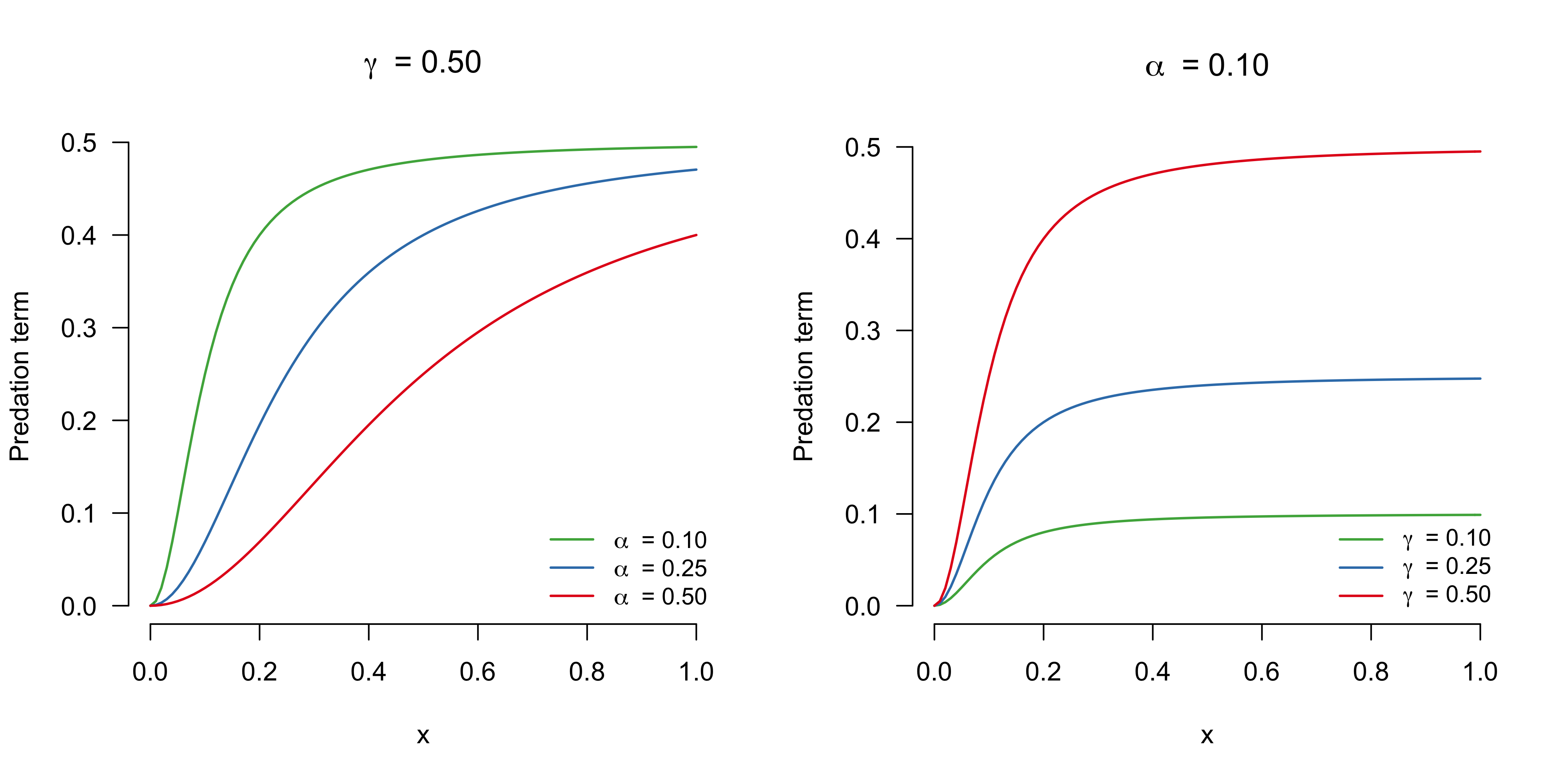
As we have discussed before, the units of the left hand side need to be the same as the units of the right hand side. As our excursion in nondimensionalization has established earlier, the logistic equation in terms of $\frac{\mathrm{d}x}{\mathrm{d}\tau}$ is dimensionless — it tells us how the population relative to carrying capacity ($x$) changes per unit of dimensionless time ($\tau$). The predation term we added also needs to be dimensionless, because summing quantities of different units is meaningless. In order for $\alpha^2 + x^2$ to make sense, $\alpha$ must also be given in population relative to the carrying capacity, that is, it must be dimensionless. The parameter $\gamma$ must be given in population relative to carrying capacity per unit of dimensionless time. We can interpret it as the maximum proportion of individuals (relative to carrying capacity) that is killed by predation that is theoretically possible (if $\alpha = 0$ and $x = 1$), per unit of dimensionless time. What a mouthful! Maybe we should have kept the original dimensions? But that would have left us with more parameters! Fearless and undeterred, we move on. For simplicity of analysis, however, we fix $\alpha = 0.10$ for the remainder of this blog post.

Now that we have the units straight, let’s continue with the analysis of the system. We are interested in finding the equilibrium points $x^{\star}$, and we could do this algebraically by solving the following for $x$:

However, we can also find the equilibrium points graphically, by visualizing both the left-hand and the right-hand side and seeing where the two lines intersect. Importantly, the intersections will depend on the parameter $\gamma$. The left panel in the figure below illustrates this for three different values of $\gamma$. For all values of $\gamma$, there exists an unstable equilibrium point at $x^{\star} = 0$. If $\gamma = 0$, then the predation term vanishes and we get back the logistic equation, which has a stable equilibrium point at $x^{\star} = 1$. For a low predation rate $\gamma = 0.10$, this stable equilibrium point gets shifted below the carrying capacity and settles at $x^{\star} = 0.89$. Astonishingly, for the intermediate value $\gamma = 0.22$, two stable equilibrium points emerge, one at $x^{\star} = 0.03$ and one at $x^{\star} = 0.68$, separated by an unstable equilibrium point at $x^{\star} = 0.29$. For $\gamma = 0.30$, the stable and unstable equilibrium points have vanished, and a single stable equilibrium point at a very low population size $x^{\star} = 0.04$ remains.

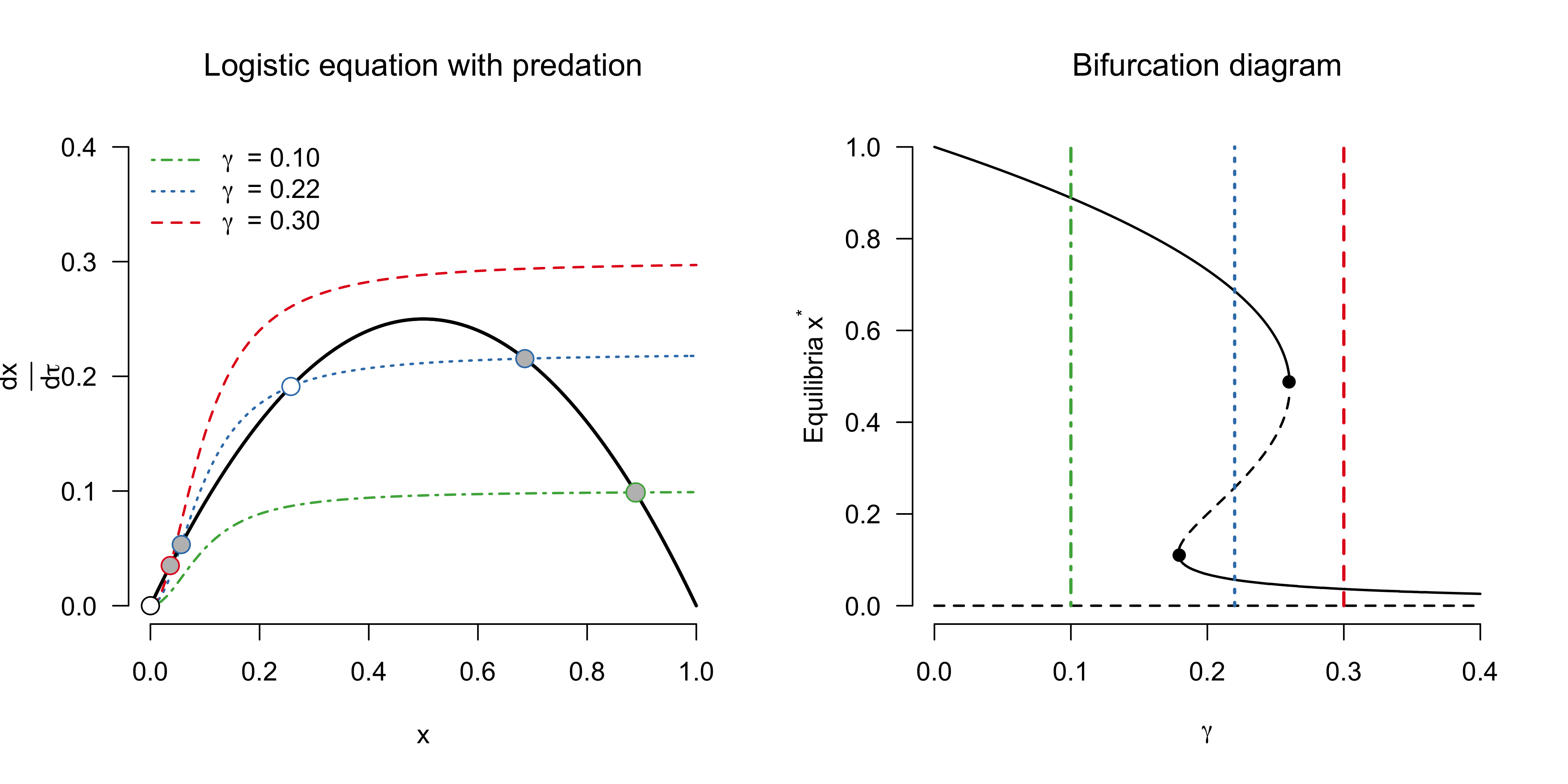
While the left panel above shows three specific values of $\gamma$, the panel on the right visualizes the stable (solid lines) and unstable (dashed lines) equilibrium points as a function of $\gamma \in (0, 0.40)$. This is known as a bifurcation diagram — it tells us the equilibrium points of the system and their stability as a function of $\gamma$. The black dots indicate the bifurcation points, that is, values of $\gamma$ at which the (stability of) equilibrium points change. For this system, we have that a stable and unstable equilibrium point collide and vanish at $\gamma = 0.18$ and $\gamma = 0.26$; while there are many types of bifurcations a system can exhibit, this type of bifurcation is known as a saddle-node bifurcation. The coloured lines indicate the three specific values from the left panel.

This simple model has a number of interesting properties that we will explore in the next sections. Before we do this, however, we look at another way to visualize the behaviour of the system.

Potentials

For unidimensional systems one can visualize the dynamics of the system in an intuitive way by using so-called “ball-in-a-cup” diagrams. Such diagrams visualize the potential function $V(x)$, which is defined in the following manner:

To solve this, we can integrate both sides with respect to $x$, which yields

where $C$ is the constant of integration, and the potential is defined only up to an additive constant. Notice that $V$ is a function of $x$, rather than a function of time $\tau$. As we will see shortly, $x$ will be the “ball” in the “cup” or landscape that is carved out by the potential $V$. Setting $C = 0$, the potential for the logistic equation with predation is given by:

The figure below visualizes the potentials for three different values of $\gamma$; since the scaling of $V(x)$ is arbitrary, I removed the $y$-axis. The left panel shows the potential for $\gamma = 0.10$, and this corresponds to the case where one unstable fixed point $x^{\star} = 0$ and one stable fixed point at $x^{\star} = 0.89$ exists. We can imagine the population $x$ as a ball in this landscape; if $x = 0$ and we add individuals to the population, then the ball rolls down into the valley whose lowest point is the stable state $x^{\star} = 0.89$.

The rightmost panel shows that under a high predation rate $\gamma = 0.30$, there are again two fixed points, one unstable one at $x^{\star} = 0$ and one stable fixed point at a very low population size $x^{\star} = 0.04$. Whereever we start on this landscape, unless $x_0 = 0$, the population will move towards $x^{\star} = 0.04$.

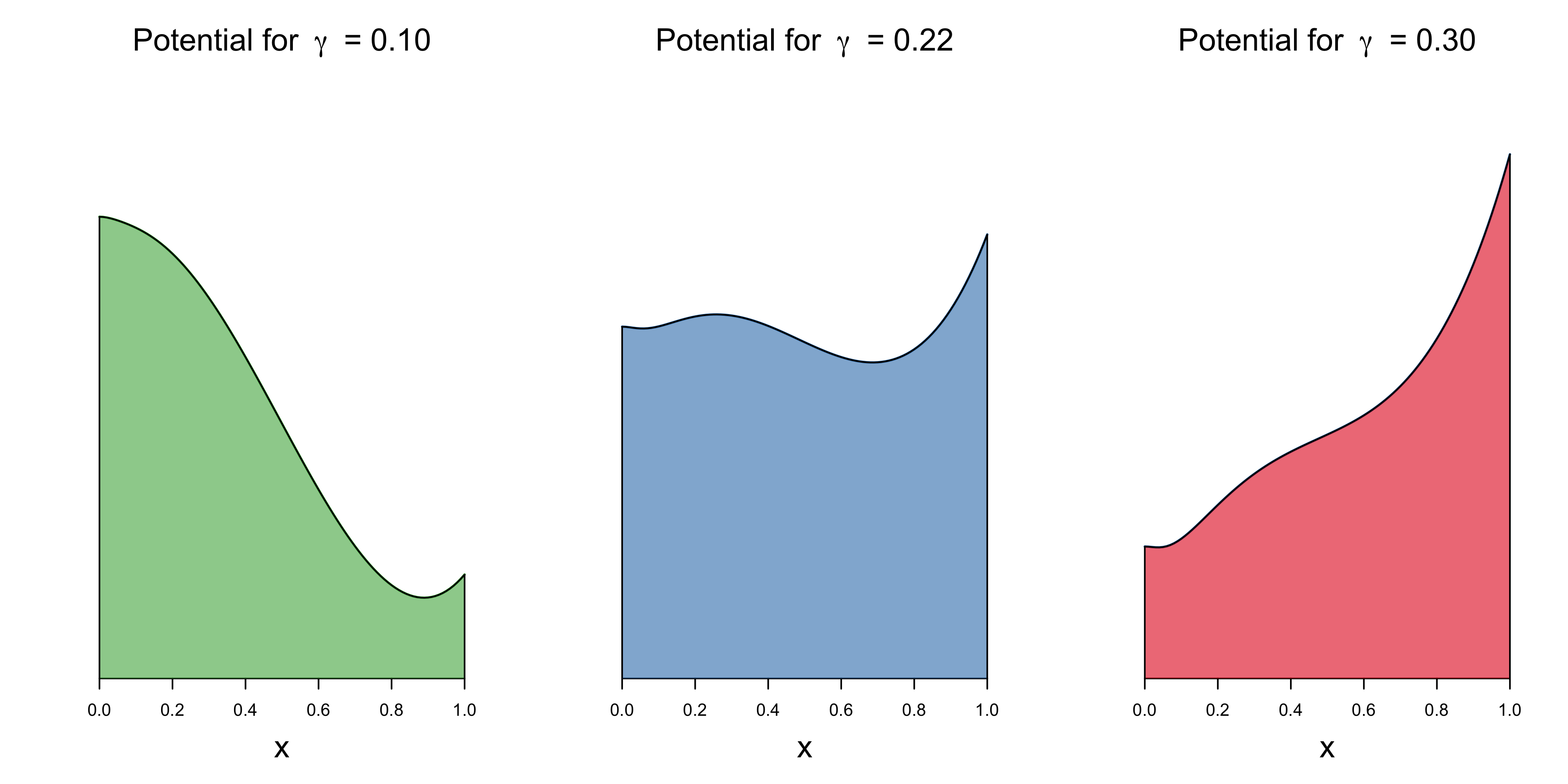
The middle panel above is the most interesting one. It shows that the potential for $\gamma = 0.22$ exhibits two valleys, corresponding to the stable fixed points $x^{\star} = 0.03$ and $x^{\star} = 0.68$. These two points are separated by a hill, corresponding to an unstable fixed point at $x^{\star} = 0.29$. Depending on the initial condition, the population would either converge to a very low or moderately high stable size. For example, if $x_0 = 0.25$, then we would “roll” towards the left, into the valley whose lowest point corresponds to $x^{\star} = 0.03$. On the other hand, if $x_0 = 0.40$, then individuals can procreate unabated by predation and reach a stable point at $x^{\star} = 0.68$.

Visualizing potentials as “ball-in-a-cup” diagrams is a wide-spread way to communicate the ideas of stable and unstable equilibrium points. But they suffer from a number of limitations, and they are a little bit of a gimick. Potentials generally do not exist for higher-dimensional systems (see Rodríguez-Sánchez, van Nes, & Scheffer, 2020, for an approximation).

A necessary requirement for a system to exhibit multiple stable states are positive feedback mechanisms (e.g., Kefi, Holmgren, & Scheffer 2016). In our example, it may be that, at a sufficient size, individuals in the population can coordinate so as to fight predators better. This would allow them to grow towards the higher stable population size. Below that “coordination” point, however, they cannot help each other efficiently, and predators may have an easy time feasting on them — the population converges to the smaller stable population size. This constitutes an Allee effect.

Systems that exhibit multiple stable states can show critical transitions between them. These transitions are not only notoriously hard to predict, but they can also be hard to reverse, as we will see in the next section.

Critical transitions and hysteresis

What happens if we slowly increase the extent of predation in our toy model? To answer this, we allow for a slowly changing $\gamma$. Formally, we add a differential equation for $\gamma$ to our system:

where $\beta > 0$ is a constant. In contrast to the first model we studied, $\frac{\mathrm{d}\gamma}{\mathrm{d}\tau}$ does not itself depend on $\gamma$, and hence will not show exponential growth. Instead, its rate of change is constant at $\beta$, and so $\gamma(\tau)$ is a linear function with slope given by $\beta$.

Note further that the differential equation for $\gamma$ does not feature a term that depends on $x$, which means that it is not influenced by changes in the population size. The differential equation for $x$ obviously includes a term that depends on $\gamma$, and so the population size will be influenced by changes in $\gamma$, as we will see shortly. We can again numerically approximate the system reasonably well when choosing $\Delta_t$ to be small. We add small additive perturbations to $x$ at each time step, writing:

where $f$ is the logistic equation with predation and $\varepsilon_n \sim \mathcal{N}(0, \sigma)$.⁶ We implement this in R as follows:

solve_err <- function(
  f, beta, x0, gamma0, delta_t = 0.01,
  nr_iter = 1000, sigma = 0.0001
) {
  
  xt <- rep(x0, nr_iter)
  gammat <- rep(gamma0, nr_iter)
  
  for (n in seq(2, nr_iter + 1)) {
    gammat[n] <- gammat[n-1] + delta_t * beta
    xt[n] <- xt[n-1] + delta_t * f(xt[n-1], gammat[n-1]) + rnorm(1, 0, sigma)
  }
  
  time <- seq(0, nr_iter * delta_t, delta_t)
  res <- cbind(time, xt, gammat)
  res
}

We treat $\gamma$ as a parameter that slowly increases from $\gamma = 0$ to $\gamma = 0.40$. We encode the fact that $\gamma$ changes slowly by setting $\beta$ to a small value, in this case $\beta = 0.004$. The average absolute rate of change of $x$ across population sizes and $\gamma \in [0, 0.40]$ is about $0.10$:

may <- function(x, gamma) x * (1 - x) - gamma * x^2 / (0.10^2 + x^2)
 
x <- seq(0, 1, 0.01)
gammas <- seq(0, 0.40, 0.01)
mean(sapply(gammas, function(gamma) mean(abs(may(x, gamma)))))

## [1] 0.09725383

and so $x$ changes about $0.10 / 0.004 = 25$ times faster than $\gamma$ on average. Systems where one component changes quickly and the other more slowly are called fast-slow systems (e.g., Kuehn, 2013). The code simulates one trajectory that we will visualize below.

delta_t <- 0.01
nr_iter <- 10000
 
set.seed(1)
res <- solve_err(
  f = may, beta = 0.004, x0 = 1, gamma0 = 0,
  nr_iter = nr_iter, delta_t = delta_t, sigma = 0.001
)

As a reminder, the left panel in the figure below shows the bifurcation diagram for the logistic equation with predation. The right panel shows a critical transition. In particular, the solid black line shows the time-evolution of the population starting at carrying capacity $x_0 = 1$. We slowly increase the predation rate from $\gamma = 0$ up to $\gamma = 0.40$, as the solid blue line indicates. The population size decreases gradually as we increase $\gamma$, and this closely follows the bifurcation diagram on the left. At the bifurcation point $\gamma = 0.26$, however, the population size crashes down to very low levels.

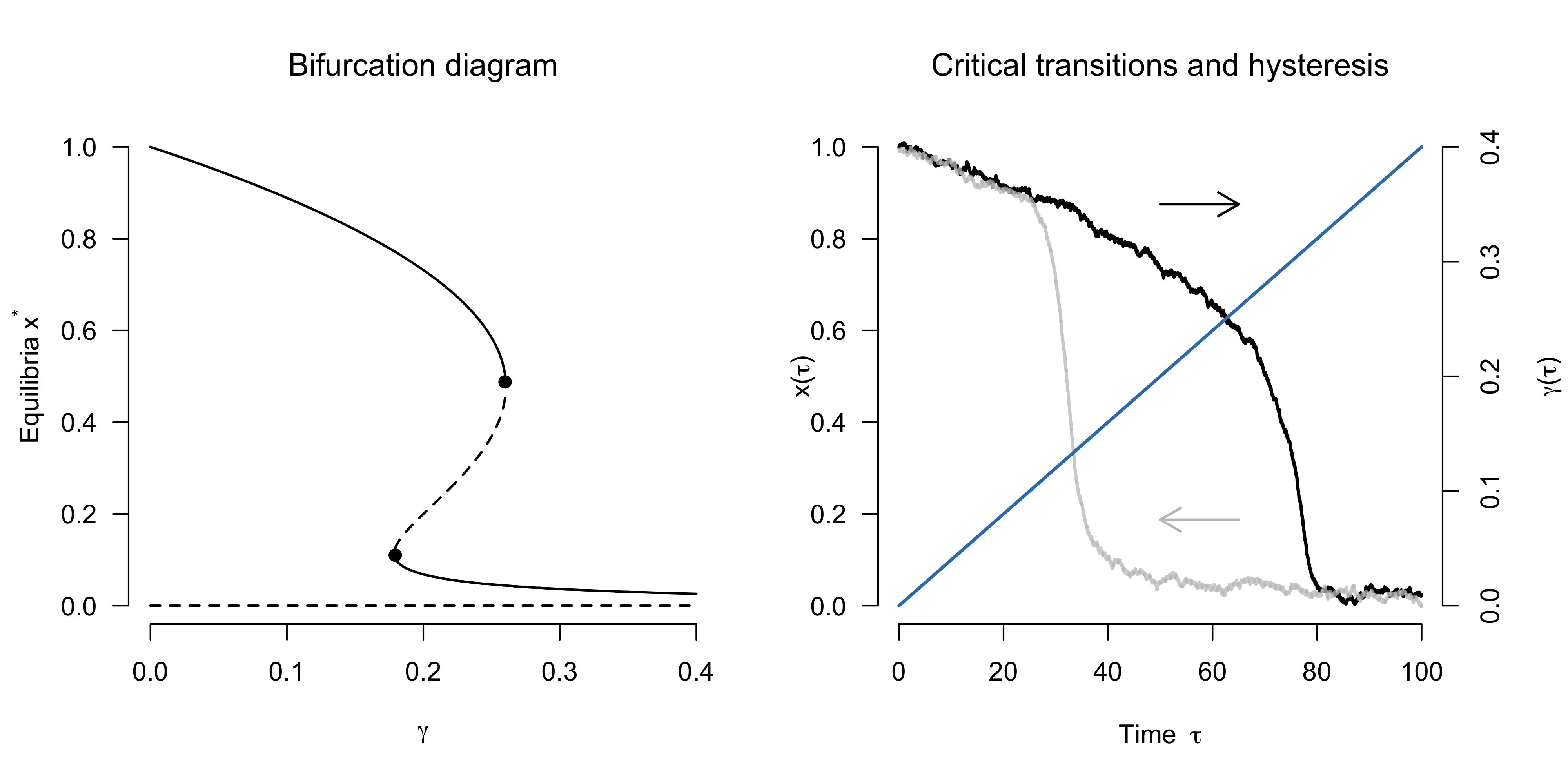
Can we recover the population size by decreasing $\gamma$ again? We can, but it requires substantially more effort! The solid gray line indicates the trajectory starting from a low population size and a high predation rate $\gamma = 0.40$. We reduce $\gamma$, but we have to reduce it all the way to $\gamma = 0.18$ for the population to then suddenly recover again. The phenomenon that a transition may be hard to reverse in this specific sense is known as hysteresis.

In the time-series above, we see that the system moves eratically around the equilibrium — after perturbations which push the system out of equilibrium, it is quick to return to equilibrium. Importantly, changes in $\gamma$ affect the equilibrium of the system itself. At the saddle-node bifurcation $\gamma = 0.26$, the stable equilibrium point vanishes, and the system moves towards the other stable equilibrium point that entails a much lower population size. This “crashing down” is a transient phase during which the system is out of equilibrium. How long the system takes to reach another stable equilibrium point after the one it tracked vanished depends on the nature of the system. Given the eagerness with which Escherichia coli reproduces, for example, it is a matter of mere hours until its population has recovered after predation has been sufficiently reduced. Transitions in the earth’s climate, however, may take hundreds of years.

Here, we assume that we know the equation that describes population growth under predation. For almost all real-word systems, however, we do not have an adequate model and thus may not know whether a particular system is in a transient phase, or whether the changes we are seeing are due to changes in underlying parameters that influence the equilibrium. If the system is in a transient phase, it can change without any change in parameters or perturbations, which — from a conservation perspective — is slightly unsettling (Hastings et al., 2018). Yet transients can also hold opportunities. For example, if a system that is pushed over a tipping point has a slow transient, we may still be able to intervene and nurture the system back before it crashes into the unfavourable stable state (Hughes et al., 2013).

While the simple models we look at in this blog post quickly settle into equilibrium, many real-world systems are periodically forced (e.g., Rodríguez-Sánchez, 2020; Strogatz, 2003) and may never do so. This can lead to interesting dynamics and has implication for critical transitions (e.g., Bathiany et al. 2018), but this is for another blog post.

Critical transitions — such as the one illustrated in the figure above — are hard to foresee. Looking at how the mean of the population size changes, one would not expect a dramatic crash as predation increases. In the next section, we will see how the phenomenon of critical slowing down may help us anticipate such critical transitions.

Critical slowing down

The logistic equation with predation exhibits a phenomenon called critical slowing down: as the population approaches the saddle-node bifurcation, it returns more slowly to the stable equilibrium after small perturbations. We can study this analytically in our simple model. In particular, we are interested in the dynamics of the system after a (small) perturbation $\eta(\tau)$ that pushes the system away from the fixed point. We write:

This is essentialy what we had when we simulated from the system and added a little bit of noise at each time step. The dynamics of the system close to the fixed point turn out to be the same as the dynamics of the noise. To see this, we derive a differential equation for $\eta = x - x^{\star}$:

since the rate of change at the fixed point, $\frac{\mathrm{d}x^{\star}}{\mathrm{d}\tau}$, is zero and where $f$ is the logistic equation with predation. This tells us that the dynamics of the perturbation $\eta$ is simply given by the dynamics of the system evaluated at $f(x^{\star} + \eta)$. For simplicity, we linearize this equation, writing:

since $f(x^{\star}) = 0$ and where we ignore higher-order terms $\mathcal{O}(\eta^2)$. While the symbols are different, the structure of the equation might look familiar. In fact, it is a linear equation in $\eta$, and so its solution is given by the exponential function:

where $\eta_0$ is the initial condition. Therefore, the dynamics of the system close to the fixed point $x^{\star}$ is given by:

In sum, we have derived an (approximate) equation that describes the dynamics of the system close to equilibrium after a small perturbation. As an aside, this approximation can be used to analyze the stability of fixed points: at a stable fixed point, $f’(x^{\star}) < 0$ and the system hence returns to the fixed point; at unstable fixed points, $f’(x^{\star}) > 0$ and the system moves away from the fixed point. Such an analysis is known as linear stability analysis, because we have linearized the system dynamics close to the fixed point.

We are now in a position to illustrate the phenomenon of critical slowing down. In particular, note that $\eta(\tau)$ depends on the derivative of the differential equation $f$ with respect to $x$ — denoted by $f’$ — evaluated at the fixed point $x^{\star}$. For the logistic equation with predation, we have that $f’$:

In the following, we will evaluate this function at various equilibrium points $x^{\star}$, which depend on $\gamma$, as we have seen before in the bifurcation diagram. To make this apparent, we define a new function:

where the value of $x^{\star}$ is constrained by $\gamma$.⁷ This function gives the recovery rate of the system from small perturbations close to the equilibrium. The code for this function is:

lambda <- function(xstar, gamma) 1 - 2*xstar - gamma * 0.02 * xstar / (0.01 + xstar^2)^2

In order to get the equilibrium points $x^{\star}$ for a particular value of $\gamma$, we need to find the values of $x$ for which the logistic equation with predation is zero. We can do this using the following code:

library('rootSolve')
 
get_fixedpoints <- function(gamma) {
  uniroot.all(f = function(x) may(x, gamma), interval = c(0, 1))
}

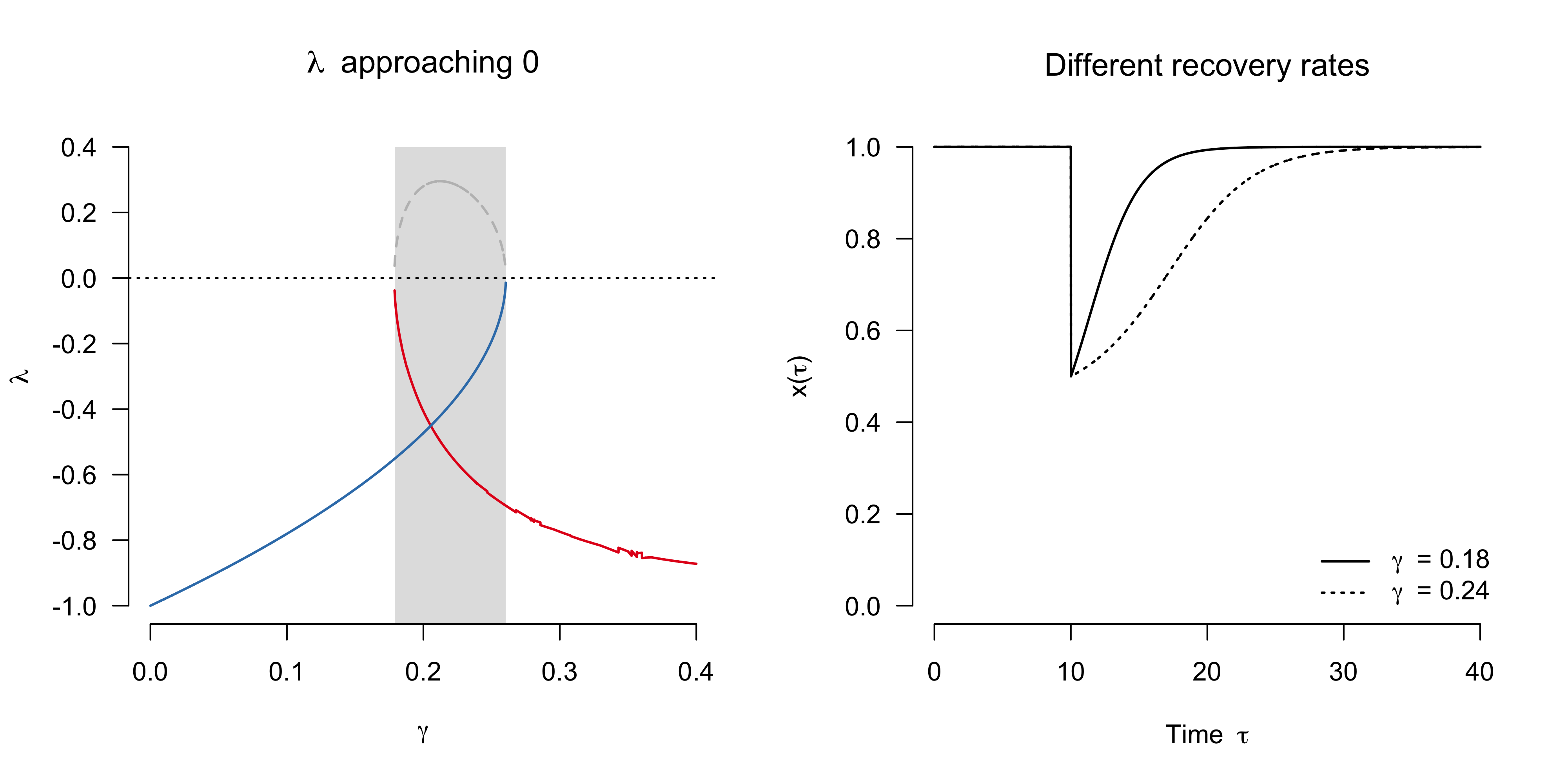
Let’s apply this on an example. The recovery rate from perturbations away from a particular fixed point $x^{\star}$ is given by $\lambda(x^{\star}, \gamma)$, and so a smaller absolute value for $\lambda$ will result in a slower recovery. Take $\gamma = 0.18$ and $\gamma = 0.24$ as examples. For these values, there are two stable fixed points, and suppose that the system is at the larger fixed point. These fixed points are given by $x^{\star} = 0.77$ and $x^{\star} = 0.63$, respectively, as the following computation shows:

rbind(
  # unstable, stable, unstable, stable
  round(get_fixedpoints(gamma = 0.18), 2),
  round(get_fixedpoints(gamma = 0.24), 2)
)

##      [,1] [,2] [,3] [,4]
## [1,]    0 0.10 0.13 0.77
## [2,]    0 0.05 0.32 0.63

We can plug these fixed points into the equation for $\lambda$, which gives us the respective rates with which these systems return to equilibrium. These are:

which can easily be verified:

rbind(
  round(lambda(x = 0.77, gamma = 0.18), 2),
  round(lambda(x = 0.63, gamma = 0.24), 2)
)

##       [,1]
## [1,] -0.55
## [2,] -0.28

Indeed, the system for which $\gamma = 0.24$ has $\lambda$ smaller in absolute value than the system for which $\gamma = 0.18$, and thus returns more slowly to equilibrium after an external perturbation.

The left panel in the figure below shows how $\lambda$ changes as a continuous function of $\gamma \in [0, 0.40]$. We see that $\lambda$ increases towards $\lambda = 0$ at the saddle-node bifurcation $\gamma = 0.26$ (when coming from the left) or $\gamma = 0.18$ (when coming from the right). The dashed gray lines indicates $\lambda > 0$, which is the case for unstable equilibrium points; in other words, perturbations do not decay but grow close to the unstable equilibrium point, and hence the system does not return to it.

The panel on the right illustrates the slower recovery rate. In particular, I simulate from these two systems and, at $\tau = 10$, half their population size. The system with $\gamma = 0.18$ recovers more swiftly to its stable equilibrium than the system with $\gamma = 0.24$.

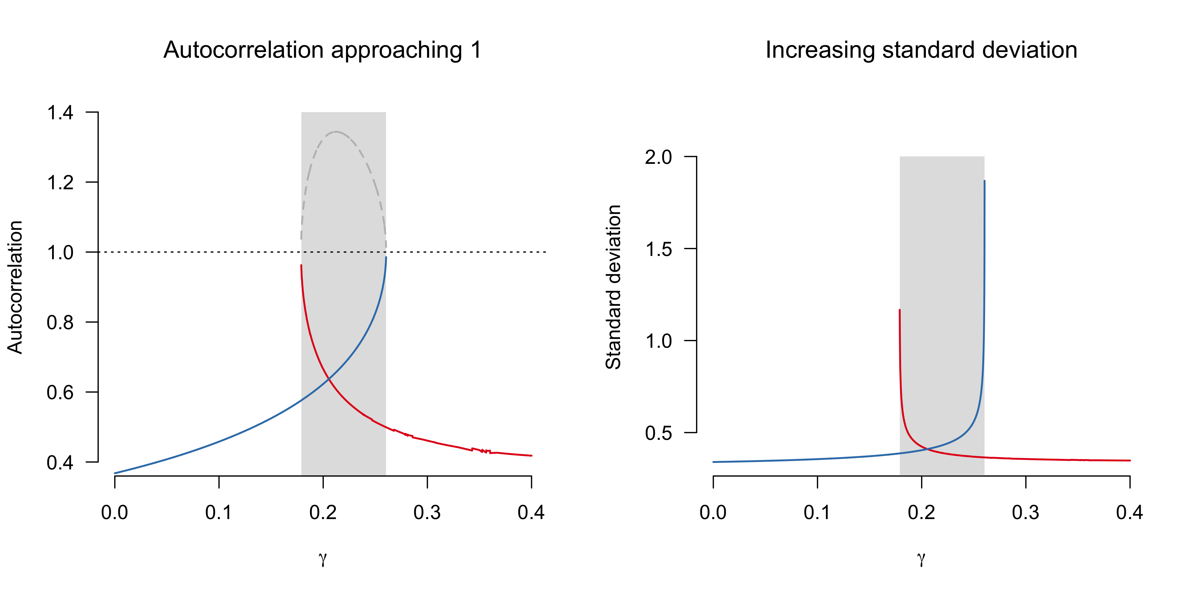
The phenomenon of critical slowing down is the basis of widely used early warning signals such as autocorrelation and variance. Indeed, one can show that the autocorrelation and variance are given by $e^{\lambda}$ and $\frac{\sigma_{\varepsilon}^2}{1 - e^{2\lambda}}$, respectively, where $\sigma_{\varepsilon}^2$ is the noise variance (see e.g. the appendix in Dablander et al., 2020). Hence, these quantities will increase as the system approaches the bifurcation point, as the figure below illlustrates.

Early warning signals based on critical slowing down have seen a surge in attention in the last two decades, with prominent review articles in ecology and climate science (e.g., Scheffer et al., 2009, 2012; Lenton, 2011). The idea of critical slowing down goes back much further, and was well-known to proponents of catastrophe theory (e.g., Zeeman, 1976); indeed, critical slowing down is one of the so-called catastrophe flags (see van der Maas et al. 2003, for an overview and an application to attitudes). Wissel (1984) (re)discovered critical slowing down in simple systems and used it to predict the extinction of a population of rotifers. The wonderful experimental demonstrations by Drake & Griffin (2010) and Dai et al. (2012) are modern variations on that theme.

Critical transitions are notoriously hard to predict, and the potential of generic signals that warn us of such transitions is vast. Early warning signals based on critical slowing down are subject to a number of practical and theoretical limitations, however — for example, they can occur prior to transitions that are not critical, and they can fail to occur prior to critical transitions. For an overview and a discussion, see Dablander, Pichler, Cika, & Bacilieri (2020).

Conclusion

Dynamical systems theory is a powerful framework for modelling how systems change over time. In this blog post, we have looked at simple toy models to elucidate some core concepts. Intriguingly, we have seen that even a very simple model can exhibit intricate behaviour, such as multiple stable states and critical transitions. Yet most interesting real-world systems are much more complex, and care must be applied when translating intuitions from low-dimensional toy models into high-dimensional reality.

I would like to thank Andrea Bacilieri, Jill de Ron, Jonas Haslbeck, and Oisín Ryan for helpful comments on this blog post.

References

• Abbott, K. C., Ji, F., Stieha, C. R., & Moore, C. M. (2020). Fast and slow advances toward a deeper integration of theory and empiricism. Theoretical Ecology, 13(1), 7-15.
• Bacaër, N. (2011). A short history of mathematical population dynamics. Springer Science & Business Media.
• Bathiany, S., Scheffer, M., Van Nes, E. H., Williamson, M. S., & Lenton, T. M. (2018). Abrupt climate change in an oscillating world. Scientific reports, 8(1), 1-12.
• Dablander, F., Pichler, A., Cika, A., & Bacilieri, A. (2020). Anticipating Critical Transitions in Psychological Systems using Early Warning Signals: Theoretical and Practical Considerations.
• Dai, L., Vorselen, D., Korolev, K. S., & Gore, J. (2012). Generic indicators for loss of resilience before a tipping point leading to population collapse. Science, 336(6085), 1175-1177.
• Drake, J. M., & Griffen, B. D. (2010). Early warning signals of extinction in deteriorating environments. Nature, 467(7314), 456-459.
• Hastings, A., Abbott, K. C., Cuddington, K., Francis, T., Gellner, G., Lai, Y. C., … & Zeeman, M. L. (2018). Transient phenomena in ecology. Science, 361(6406).
• Hughes, T. P., Linares, C., Dakos, V., Van De Leemput, I. A., & Van Nes, E. H. (2013). Living dangerously on borrowed time during slow, unrecognized regime shifts. Trends in Ecology & Evolution, 28(3), 149-155.
• Kallis, G. (2019). Limits: Why Malthus was wrong and why environmentalists should care. Stanford University Press.
• Kéfi, S., Holmgren, M., & Scheffer, M. (2016). When can positive interactions cause alternative stable states in ecosystems?. Functional Ecology, 30(1), 88-97.
• Kuehn, C. (2013). A mathematical framework for critical transitions: normal forms, variance and applications. Journal of Nonlinear Science, 23(3), 457-510.
• Lenton, T. M. (2011). Early warning of climate tipping points. Nature Climate Change, 1(4), 201-209.
• Ludwig, D., Jones, D. D., & Holling, C. S. (1978). Qualitative analysis of insect outbreak systems: the spruce budworm and forest. The Journal of Animal Ecology, 47(1), 315-332.
• May, R. M. (1977). Thresholds and breakpoints in ecosystems with a multiplicity of stable states. Nature, 269(5628), 471-477.
• Rodríguez-Sánchez, P. (2020). Cycles and interactions: A mathematician among biologists. PhD Thesis.
• Rodríguez-Sánchez, P., Van Nes, E. H., & Scheffer, M. (2020). Climbing Escher’s stairs: A way to approximate stability landscapes in multidimensional systems. PLoS Computational Biology, 16(4), e1007788.
• Scheffer, M., Bascompte, J., Brock, W. A., Brovkin, V., Carpenter, S. R., Dakos, V., … & Sugihara, G. (2009). Early-warning signals for critical transitions. Nature, 461(7260), 53-59.
• Scheffer, M., Carpenter, S. R., Lenton, T. M., Bascompte, J., Brock, W., Dakos, V., … & Pascual, M. (2012). Anticipating critical transitions. Science, 338(6105), 344-348.
• Strogatz, S. H. (2003). Sync: How Order Emerges from Chaos in the Universe. Nature, and Daily Life. Hachette Books.
• Wissel, C. (1984). A universal law of the characteristic return time near thresholds. Oecologia, 65(1), 101-107.
• Van der Maas, H. L., Kolstein, R., & Van Der Pligt, J. (2003). Sudden transitions in attitudes. Sociological Methods & Research, 32(2), 125-152.
• Zeeman, E. C. (1976). Catastrophe theory. Scientific American, 234(4), 65-83.

Footnotes