Causal effect of Elon Musk tweets on Dogecoin price

If you think of Dogecoin — the cryptocurrency based on a meme — you can’t help but also think of Elon Musk. That guy loves the doge, and every time he tweets about it, the price goes up. While we all know that correlation is not causation, we might still be able to quantify the causal effect of Elon Musk’s tweets on the price of Dogecoin. Sounds adventurous? That’s because it is! So buckle up before scrolling down.

Tanking Tesla

Elon Musk is notorious for being able to swing markets. In a great blog post from last year, Alex Hayes used the S&P500 as a control to estimate the causal effect of the tweet below on Tesla’s stock price. He used the excellent CausalImpact R package developed by Brodersen et al. (2015). I quickly reproduced his analysis, see below and the Post Scriptum.

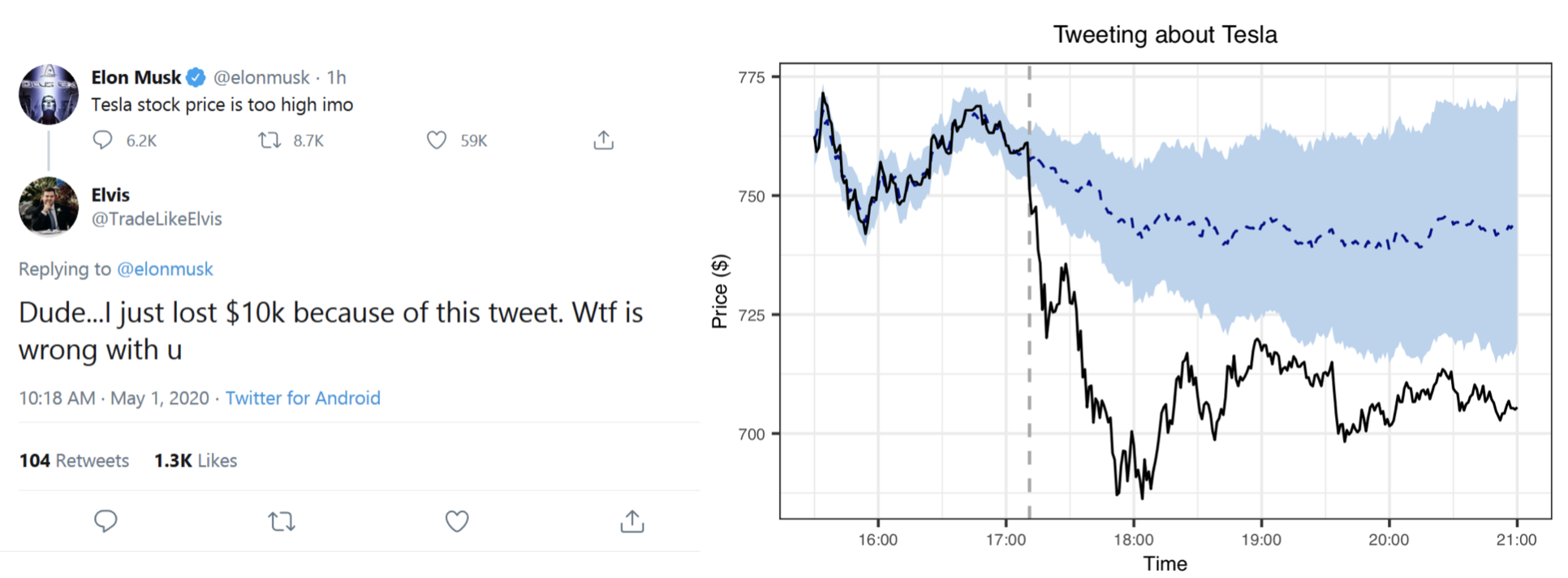
The vertical dashed line indicates the timing of Elon’s tweet, which was around 15:11 UTC, which is 16:11 CET (central European winter time) and 17:11 CEST (central European summer time). The black line gives Tesla’s stock price. The blue dashed line gives the model’s prediction of Tesla’s stock price using the S&P500 as a control (see Brodersen, 2015, for details on the model). We see that, prior to the tweet, the predictions align well with Tesla’s actual stock price. The time zone throughout the remainder of this blog post, by the way, is CET.

Using the S&P500, Alex predicted what Tesla’s share price would have been had Elon not tweeted. The difference between that prediction and the actual trajectory of Tesla’s stock price is an estimate of the causal effect. This assumes that there were no other events besides Elon’s tweet that influenced Tesla’s stock price but did not influence the S&SP500 at the time; that the tweet did not influence the S&P500 itself (Tesla was not in the S&P500 back then); that the relationship between Tesla and the S&P500 holds after the post-tweet period; and that there is no hidden variable that caused both Elon to tweet and Tesla to tank. (And, of course, that counterfactuals make sense.)

Moonshooting Dogecoin: Part I

Let’s turn to the recent Dogecoin mania. The figure below shows the price of Dogecoin and Bitcoin for a selected period of time (see the Post Scriptum for how to get the data).

Dogecoin exploded that week, largely because Redditors rallied around it after shooting GameStop to the moon. There are currently about 18 million Bitcoins in circulation, and there is a maximum supply of 21 million. There are about 127 billion Dogecoins in circulation, and in contrast to Bitcoin, there is no upper limit to what that number can be.

To better compare the two time-series, we standardize them (with respect to themselves) in the figure below.

We see that Bitcoin is more volatile at the beginning, but that both cryptocurrencies increase starting at around 28th January 12:00. The vertical black line indicates the time Elon Musk fired off a tweet. What did he share with the world?

Haha, that’s great stuff … what’s the causal effect of this tweet? Since the S&P500 is in quite a different class than cryptocurrencies, I use Bitcoin to predict the counterfactual Dogecoin price. I use a subset of the above data, starting from 12:00 on the 28th of January, as Bitcoin does not track Dogecoin particularly well before. Similarly, I only look at a subset of the data after the tweet. This is because cryptocurrencies are extremely volatile, and the causal effect of Elon Musk’s tweet may thus wash out rather quickly.

Using the wonderful CausalImpact R package, we get the following result (see also the Post Scriptum).

We see that the model predicts the price of Dogecoin reasonably well prior to Elon’s tweet. The counterfactual Dogecoin price (that is, the price of Dogecoin had Elon not tweeted) is predicted to stay rather flat, while the actual price rises. Yet it does not rise immediately, but with a delay — maybe because he tweeted in the middle of the night? In any event, Dogecoin showed an average increase of 33% (with a 95% credible interval ranging from 23% to 42%), but note that this estimate naturally depends on the post-tweet time frame we consider. In particular, the previous figure showed that the Dogecoin price dips after the initial increase. Overall, however, it does seem that Elon’s tweet had a substantial causal effect on the price of Dogecoin.

Recall that the analysis assumes that there were no other events at the time that selectively influenced Dogecoin but not Bitcoin. However, Redditors rallied around the cryptocurrency at the same time, very likely confounding the tweet’s causal effect. Luckily for us, Elon struck twice.

Moonshooting Dogecoin: Part II

A week after the initial frenzy, Musk fired off a series of tweets about Dogecoin. Let’s zoom in on the data.

The vertical black line indicate the time of the first of Elon’s tweets, after which several others followed. What insights can we glean from them?

Cool, cool. Dogecoin rose substantially after this avalance of tweets. But again, this does not mean Elon’s tweets caused the price to rise. To assess whether these tweets had a causal effect, I employ the same analysis as above. Since Musk tweeted several times, I take the first tweet as the reference point. Similar to above, I only select a subset of the data, this time starting from 3th February 12:00.

The average causal effect estimate is a price increase of 23%, with a 95% credible interval between 19% and 28% (but note again that this is sensitive to the extent of the post-tweet time period we consider). There is little delay between the first tweet and the price rise, and Redditors rallying around Dogecoin is not as big of a concern as it was previously. But the counterfactual predictions seem somewhat less convincing than before, reflecting the rather poor correlation between Dogecoin and Bitcoin pre-tweet. The method naturally acounts for uncertainty (for details, see Brodersen et al., 2015).

Conclusion

Causal inference always comes with assumptions. Here, we asssumed that there was no other event that influenced the price of Dogecoin but not the price of Bitcoin at the time of Elon Musk’s tweets, and that there was no third variable that caused both Musk to tweet and Dogecoin to rise. These assumptions seem more plausible in the second analysis than in the first.

We also assumed that Bitcoin prices track Dogecoin prices reasonably well, and that the relation persists after the tweets. One could sanity-check how suitable Bitcoin is as a control by running the analysis on various subsets of the data, and comparing the predicted Dogecoin price with the actual Dogecoin price. But since there is only so much time I want to spend thinking about Dogecoin on a Sunday afternoon, I leave this validation to others.

One could probably come up with a better control by combining several different cryptocurrencies instead of relying only on Bitcoin — or drop the whole control spiel and slap a Gaussian process on the doge in an interrupted time-series manner (e.g., Leeftink & Hinne, 2020). On a more philosophical note, the analysis assumes that counterfactual statements make sense, which is not uncontroversial (e.g., Dawid, 2000; Peters, Janzing, & Schölkopf, 2017, p. 106).

The analysis further assumes that Bitcoin prices are not influenced by Musk’s tweets. If they were influenced by them — say they cause a rise in Bitcoin prices — then the causal effect on Dogecoin would be downward biased. It seems likely that Musk’s tweets, if they were to influence Dogecoin, would also influence Bitcoin (e.g., simply by drawing attention to cryptocurrencies), and so if one were really interested in an unbiased — or rather, less biased — estimate, one would have to think harder.

Elon Musk has 46 million Twitter followers, and while I would not trust the precise causal effect estimates we arrived at in this blog post, it seems pretty plausible to me that he could influence the price of Dogecoin by mere key strokes. I don’t think, however, that this is a good thing.

I would like to thank Andrea Bacilieri for very helpful comments on this blog post.

Post Scriptum

The code below gets the relevant data sets from Tiingo using the riingo R package. This requires an API key, but you can download the data from here (for the Tesla re-analysis) and here and here (for the two Dogecoin analyses) in case you do not want to create an account.

Tesla Analysis

The code below reproduces the analysis by Alex Hayes. Note that Musk tweeted in May, in which central Europe is in summer time (CEST), which is UTC+02:00 and not UTC+01:00 … don’t get me started.

library('dplyr')
library('riingo')
library('ggplot2')
library('CausalImpact')
 
# riingo uses UTC
# CET is UTC+01:00
# CEST is UTC+02:00
# Musk tweeted during summer time
start <- as.POSIXct('2020-05-01 11:00:00 UTC', tz = 'UTC')
end <- as.POSIXct('2020-05-01 19:00:00 UTC', tz = 'UTC')
tweet <- as.POSIXct('2020-05-01 15:11:00 UTC', tz = 'UTC')
 
tesla <- riingo_iex_prices(
  'TSLA', start_date = '2020-05-01',
  end_date = '2020-05-01', resample_frequency = '1min'
  ) %>% filter(date <= end)
 
sp500 <- riingo_iex_prices(
  'SPY', start_date = '2020-05-01',
  end_date = '2020-05-01', resample_frequency = '1min'
) %>% filter(date <= end)
 
times <- tesla$date
tweet_ix <- which(times == tweet)
tofit <- zoo(cbind(tesla$close, sp500$close), times)
 
fit <- CausalImpact(tofit, times[c(1, tweet_ix)], times[c(tweet_ix + 1, length(times))])
plot(fit, 'original') +
  xlab('Time') +
  ylab('Price ($)') +
  ggtitle('Tweeting about Tesla') +
  theme(
    axis.text = element_text(size = text_size),
    axis.title = element_text(size = axis_size),
    plot.title = element_text(size = title_size, hjust = 0.50)
  )

Dogecoin Analysis

The code below gets the data set.

get_data <- function(start_date, end_date) {
  
  # Get Bitcoin in euros
  bit <- riingo_crypto_prices(
    'btceur', start_date = start_date,
    end_date = end_date, resample_frequency = '1min'
  ) %>% mutate(crypto = 'Bitcoin')
 
  # We get Dogecoin in Bitcoin, then convert it to euros
  doge <- riingo_crypto_prices(
    'dogebtc', start_date = start_date,
    end_date = end_date, resample_frequency = '1min'
  ) %>% mutate(crypto = 'Dogecoin')
  
 
  # Join data frames (and keep only rows where we have dogecoin and bitcoin data)
  dat <- full_join(doge, bit) %>% 
    group_by(date) %>% 
    mutate(
      n = n(),
      price = close,
      crypto = factor(crypto, levels = c('Dogecoin', 'Bitcoin'))
    ) %>% 
    filter(n == 2)
  
  # Convert dogecoin price to be relative euro, not relative to bitcoin
  dat[dat$crypto == 'Dogecoin', ]$price <- (
    dat[dat$crypto == 'Dogecoin', ]$close * dat[dat$crypto == 'Bitcoin', ]$close
  )
  
  dat
}
 
# dat <- get_data(start_date = '2021-01-27', end_date = '2021-01-30')
dat <- read.csv('http://fabiandablander.com/assets/data/doge-data-1.csv') %>% 
  mutate(
    date = as.POSIXct(date, tz = 'UTC')
  )

The analysis code for the causal effect of the first tweet is shown below.

tweets <- as.POSIXct(
  c(
  '2021-01-28 22:47:00 UTC',
  '2021-02-04 07:29:00 UTC',
  '2021-02-04 08:15:00 UTC',
  '2021-02-04 07:57:00 UTC',
  '2021-02-04 08:27:00 UTC'
  ), tz = 'UTC'
)
 
fit_model <- function(datsel, tweet_time) {
  doge <- filter(datsel, crypto == 'Dogecoin')
  bit <- filter(datsel, crypto == 'Bitcoin')
  
  times <- doge$date
  tofit <- zoo(cbind(doge$price, bit$price), times)
  
  tweet_ix <- which(times == tweet_time)
  fit <- CausalImpact(
    tofit, times[c(1, tweet_ix)], times[c(tweet_ix + 1, length(times))]
  )
  
  fit
}
 
# Select subset of data for analysis
start_analysis <- as.POSIXct('2021-01-28 11:00:00 UTC', tz = 'UTC')
end_analysis <- as.POSIXct('2021-01-29 01:00:00 UTC', tz = 'UTC')
datsel <- filter(dat, between(date, start_analysis, end_analysis))
 
fit1 <- fit_model(datsel, tweets[1])
plot(fit1, 'original') +
  xlab('Time') +
  ylab('Price (€)') +
  ggtitle('Tweeting about Dogecoin (28th January)') +
  theme(
    axis.text = element_text(size = text_size),
    axis.title = element_text(size = axis_size),
    plot.title = element_text(size = title_size, hjust = 0.50)
  )

The analysis code for the causal effect of the later avalanche of tweets is shown below. For some reason, riingo has lots of missing data during that time period. Thus I downloaded the cryptocurrency data from here.

dat2 <- read.csv('https://fabiandablander.com/assets/data/doge-data-2.csv') %>% 
  mutate(
    date = as.POSIXct(date, tz = 'UTC')
  )
 
# Select subset of data for analysis
start_analysis2 <- as.POSIXct('2021-02-03 12:00:00 UTC', tz = 'UTC')
end_analysis2 <- as.POSIXct('2021-02-04 10:00:00 UTC', tz = 'UTC')
datsel2 <- filter(dat2, between(date, start_analysis2, end_analysis2))
 
fit2 <- fit_model(datsel2, tweets[2])
 
plot(fit2, 'original') +
  xlab('Time') +
  ylab('Price (€)') +
  ggtitle('Tweeting about Dogecoin (4th February)') +
  theme(
    axis.text = element_text(size = text_size),
    axis.title = element_text(size = axis_size),
    plot.title = element_text(size = title_size, hjust = 0.50)
  )